Chapter 12 Optimization Workbook

12.1 What Is Optimization?

Optimization is the process of finding the best possible outcome in a system with limits or tradeoffs. In environmental science, we often want to maximize something beneficial or minimize something harmful, all while respecting ecological, physical, or budget constraints.

12.1.1 Key Ideas

A decision variable:
The thing we can change (e.g., planting density, harvest rate, flow release, fertilizer amount).
An objective function $f(x)$:
A mathematical expression that links our decision variable $x$ to the environmental outcome we care about.
A goal:
Either to maximize (e.g., carbon uptake, yield, biodiversity) or minimize (e.g., pollution, cost, heat stress).
Constraints:
The natural or practical limits that shape the feasible range of $x$.
Tradeoffs:
Improving one outcome often reduces another; optimization finds the most effective balance.
Derivatives as tools:
- $f'(x)$ shows where the function is increasing or decreasing.
- Critical points (where $f'(x)=0$) are candidates for max/min.
- $f''(x)$ helps determine whether those points are peaks or valleys.
Interpretation in context:
The mathematical optimum must be evaluated in ecological, ethical, and practical terms.

12.1.2 Why It Matters in Environmental Sciences

Optimization helps us answer questions like:

What management strategy gives the highest benefit with the lowest impact?
How do we use limited resources most efficiently?
Where is the “sweet spot” that balances productivity, cost, and sustainability?

In short, optimization allows us to make informed, mathematically justified decisions in complex environmental systems.

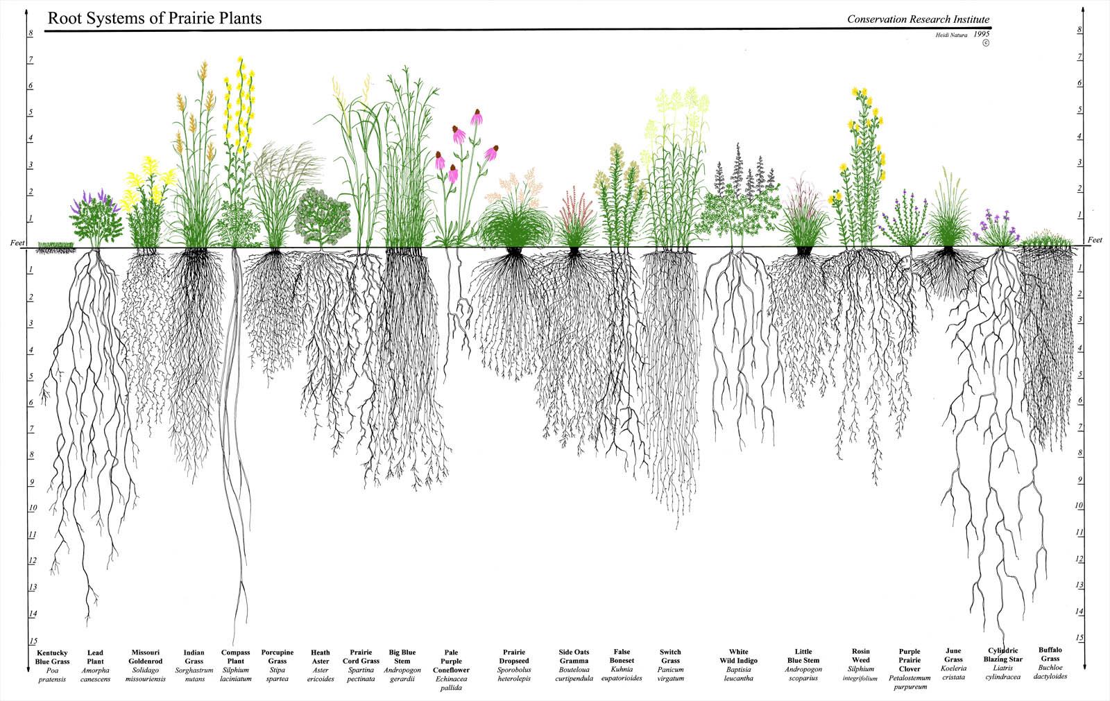
12.2 Optimization Around Us (under us)

Plants

This is an image of different rooting profiles of Prairie Plants

What might these plants be optimizing?

root profile of plants

Structures

What do you notice about these structures? historical housing structures

What is the Opimtal shape

Before we can answer this - we need to ask the question what are we optimizing for?

12.3 Qualitative Optimizating

Qualitative Case Study — Finding the Optimal Amount of Sleep

Everyone knows that sleep matters.
But the relationship between hours of sleep and how well you function the next day is not linear.

Too little sleep leaves you exhausted.
Too much sleep can make you groggy or unfocused or perhaps not enough time to do what needs to get done.
Somewhere in the middle is your personal “sweet spot.”

The goal of this activity is to help you think like an optimizer before we introduce any formulas.

1. Daily Experience (No math yet)
Think about a typical night of sleep. Describe, in your own words, what happens when you get:

Very little sleep (0–3 hours):
____________________
A moderate amount of sleep (6–9 hours):
____________________
Excessive sleep (11–14 hours):
____________________

2. What are we optimizing?
In this situation:

What is the decision variable (the thing you can adjust)?
______________
What is the outcome you care about (the “objective”)?

______________
Are you trying to maximize or minimize this outcome?
______________

3. Describe the general shape
Based on your lived experience, sketch how “next-day functioning” should change as sleep hours increase.

4. Identify the “optimal point” qualitatively

Where (roughly) do you think the maximum occurs for you?
_____ hours
Why does performance fall again after too much sleep?
___________________

5. Reflection (one sentence)
Write a single sentence that captures the idea behind optimization using the sleep example:
__________________

Qualitative Case Study — Allocating Study Time Between Two Classes to Optimize GPA

Imagine you are taking two classes this quarter.
You start with different grades in each class, and you have limited study time.
Your goal is to decide how to split your study hours to get the highest possible GPA.

This activity helps you think about optimization through a real student-centered decision.

1. Your starting point (no math yet)
Suppose:

In Class A, you’re starting strong. Your current grade already reflects good understanding.
In Class B, you’re struggling more. Your current grade is lower and needs improvement.

Fill in your own version:

Starting grade in Class A:
_____%
Starting grade in Class B:
_____%

2. What can you control?
You cannot instantly change your grades, but you can change how you distribute your time.

What is your decision variable here?
________
Are there one or two decision variables? Explain:
________
What is the outcome you want to optimize?
(Examples: GPA, average grade, exam performance)
________

3. Think about the tradeoffs
Studying more in one class usually means less time for the other. Consider:

If you spend almost all your time on Class A, what happens to Class B?
________
If you focus heavily on Class B, what happens to Class A?
________
Why might neither extreme be optimal?
________

4. Describe the “shape” of each class’s improvement curve
Imagine the effect of study hours on each class:

Class A:

You already understand the material.
Extra study helps, but each additional hour helps less (diminishing returns).
Describe the curve qualitatively:
_________

Class B:

You’re behind at the start.
The first few hours help a lot, but the benefits eventually level off.
Describe the curve qualitatively:
_________

5. Putting the system together
You have a fixed number of study hours, say 10 hours.
Let:

$x$ = hours you spend on Class B
$10 - x$ = hours you spend on Class A

Without writing formulas, describe how you could:

Represent how your grade in Class A depends on $10 - x$:
_________
Represent how your grade in Class B depends on $x$:
_________
Combine the two grades to get an overall GPA:
_________

6. Identify where the optimum might occur
Using only reasoning (no calculations):

If Class B has more “room to grow,” will you likely spend more time there or less? Why?
________
If Class A’s grade cannot change much no matter how much you study, is it worth giving it many hours?
________
Explain in one sentence where the “balanced” point might be:
________

Qualitative Case Study — Optimizing Your Thanksgiving Plate

Thanksgiving comes with a beautiful problem:
there is more good food than you can (or should) eat.
Your goal is to build the best possible plate given your limited appetite.

1. Your starting situation

You arrive at the table, and you see:

Turkey/Tofurkey
Mashed potatoes
Stuffing
Sweet potatoes
Rolls
Cranberry sauce
Green beans
Pumpkin pie

You can’t fit everything in large portions, and you can’t eat unlimited calories.

Describe your favorite dishes:
__________

Describe dishes you like less:
__________

2. What are you trying to optimize? State your objective in one sentence:
__________

3. What is your decision variable?

You must distribute a limited amount of stomach space (or calories) across different foods.

What variable(s) can you control?

In your own words, describe your main decision variable(s):
__________

4. The tradeoffs

Think through what happens as you change portions:

Fill in these intuitively:

If I eat too little, I feel:
________
If I eat too much, I feel:
________
If I only choose one dish, I feel:
________

5. Sketch the “enjoyment curve”

Without math, draw a rough graph of:

Amount of food eaten
Overall enjoyment

Your curve should show:

______________________

6. Qualitatively find the “optimal plate”

Using reasoning only:

Which foods give high enjoyment per bite?
________
Which foods give low enjoyment per bite?
________
Which foods fill you up fastest (stuffing, rolls)?
________
Which foods give you enjoyment without making you too full (cranberry sauce, green beans)?
________

Now describe your optimal combination in words:
__________

12.4 Optimization Case Studies

Case Study 1 — Optimal Nutrient Input for Algal Growth (Unconstrained)

In a controlled lake experiment, researchers add a nutrient solution (nitrogen + phosphorus mix) at rate $x$ grams per day.
For small additions, algae grow rapidly.
But after a point, adding more nutrients leads to self-shading and oxygen depletion, which reduce productivity.

A simple model for daily algal biomass produced (in grams) is:

\[ G(x) = 15x - 0.3x^2. \]

This model has no constraints: any non-negative $x$ is allowed in the experimental design.

Your Tasks

1. Understand the model
a) What is the decision variable?
b) What is the objective?
c) Is this a maximization or a minimization problem?

2. Find the optimum
Compute the derivative:

\[ G'(x) = \quad\_\_\_\_\_\_\_\_\_\_\_\_\_ \]

Find the critical point(s) by solving:

\[ G'(x) = 0. \]

Critical point(s):
\[ x = \quad\_\_\_\_\_\_\_ \]

3. Classify the critical point

Use one of the following:

First derivative sign chart
Second derivative test

Second derivative:
\[ G''(x) = \quad\_\_\_\_\_\_\_\_\_\_ \]

Is the critical point a: - local maximum?
- local minimum?
- neither?

Explain your reasoning:
_______________________

4. Interpret the result

What nutrient level $x$ gives maximum algal growth?
Plug it into $G(x)$ to compute the maximum biomass.

\[ G(x^{*}) = \quad\_\_\_\_\_\_\_\_\_\_ \]

In ecological terms, why does productivity eventually decline at high nutrient levels?

5. Reflection (one sentence)
Summarize the tradeoff revealed by this model:
___________________

Case Study 2 — Optimal Light Intensity for Photosynthesis (Unconstrained)

In a greenhouse experiment, researchers control the intensity of artificial light reaching a plant canopy.
At low light levels, photosynthesis increases rapidly.
At high light levels, enzymes saturate and heat stress reduces efficiency.

A simple model for photosynthetic rate (in µmol CO₂ m⁻² s⁻¹) as a function of light intensity $I$ (in arbitrary light units) is:

\[ P(I) = 40I - 0.5I^2. \]

There are no constraints on the light intensity: the researchers can set $I$ to any non-negative value.

Your Tasks

1. Understand the model
a) What is the decision variable?
b) What is the objective?
c) Is this a maximization or minimization problem?

2. Find the optimum
Compute the derivative:

\[ P'(I) = \quad\_\_\_\_\_\_\_\_\_\_\_\_\_ \]

Find the critical point(s) by solving:

\[ P'(I) = 0. \]

Critical point(s):
\[ I = \quad\_\_\_\_\_\_\_ \]

3. Classify the critical point

Use either:

First derivative sign chart
Second derivative test

Second derivative:
\[ P''(I) = \quad\_\_\_\_\_\_\_\_\_\_ \]

Is the critical point a:

local maximum?
local minimum?
neither?

Explain your reasoning:
___________________

4. Interpret the result

What light intensity $I$ gives the maximum photosynthetic rate?
Compute the maximum value:

\[ P(I^\*) = \quad\_\_\_\_\_\_\_\_\_\_ \]

Ecologically, why does photosynthesis decline when light becomes too intense?

5. Reflection (one sentence)
Summarize the biological tradeoff revealed by this model:
___________________

Quantitative Case Study 3 — Maximizing Volume with a Fixed Surface Area (Square Base)

You are designing an open-topped water container for a restoration project.
The container will have a square base, and you have 2 square meters of material available to build the base and the four sides.
Because the container has no lid, only the bottom and four vertical walls use material.

Let

$x$ = length of one side of the square base
$H$ = height of the container

Your goal is to build the container with the maximum possible volume

🚩 Lifeguard Optimization Problem — Rescue Path Minimization

A lifeguard stands on the shoreline at point A.
A swimmer is in distress 100 meters down the beach and 100 meters offshore at point B.

The lifeguard can:

Run on sand at: $v_r = 6 \text{ m/s}$
Swim in water at: $v_s = 2 \text{ m/s}$

The lifeguard chooses a point C, located $x$ meters down the beach, where they will enter the water and begin swimming.

Tasks

Write down the time function $T(x)$ using the distances and speeds provided.
Differentiate $T(x)$ and set the derivative equal to zero to find the critical point.
Solve for the optimal water-entry point $x$ that minimizes the total rescue time.
Interpret the result: Why is it optimal for the lifeguard to run farther down the beach before entering the water?

Activity: Which Shape Maximizes Volume When Surface Area = 100?

You are designing a container for an environmental monitoring project.
You have exactly 100 units² of construction material.
Your goal is to determine which shape produces the maximum possible volume using that fixed surface area.

You will compare three shapes:

Sphere
Closed Cylinder (top and bottom included)
Rectangular Prism with a square base

Work through each part, then compare your results at the end.

Part 1 — Sphere

A sphere of radius $r$ has:

\[ A = 4\pi r^2 = 100, \qquad V = \frac{4}{3}\pi r^3. \]

Tasks

Solve for $r$.
Compute the volume.

Solution

Surface area

\[ 4\pi r^2 = 100 \Rightarrow r = \frac{5}{\sqrt{\pi}}. \]

Volume

\[ V = \frac{4}{3}\pi \left(\frac{5}{\sqrt{\pi}}\right)^3 = \frac{500}{3\sqrt{\pi}} \approx 94.1. \]

Part 2 — Cylinder

A cylinder with radius $r$ and height $h$ has:

\[ A = 2\pi r^2 + 2\pi r h = 100, \qquad V = \pi r^2 h. \]

Tasks

Solve the surface-area constraint for $h$.
Substitute into $V$.
Optimize to find $r$ and $h$.
Compute the max volume.

Solution

Constraint

\[ h = \frac{100 - 2\pi r^2}{2\pi r}. \]

Volume

\[ V(r)=50r - \pi r^3. \]

Derivative

\[ V'(r)=50 - 3\pi r^2 = 0 \Rightarrow r=\sqrt{\frac{50}{3\pi}}\approx 2.304. \]

Height

\[ h=\frac{100}{3\pi r} \approx 4.61. \]

Volume

\[ V \approx 76.9. \]

Part 3 — Rectangular Prism (s

Let the base be $x \times x$ and the height be $h$:

\[ A = 2x^2 + 4xh = 100, \qquad V = x^2 h. \]

Tasks

Solve the constraint for $h$.
Substitute into $V(x)$.
Optimize to find $x$ and $h$.
Compute the max volume.

Solution

\[ h = \frac{100 - 2x^2}{4x}. \]

\[ V(x)=25x - \frac{1}{2}x^3. \]

\[ V'(x)=25 - \frac{3}{2}x^2 = 0 \Rightarrow x=\sqrt{\frac{50}{3}}\approx 4.083. \]

\[ h \approx 4.08. \]

\[ V \approx 68.0. \]

Part 4 — Final Comparison

Shape	Maximum Volume
Sphere	94.1
Cylinder	76.9
Rectangular Prism	68.0

Conclusion:
The sphere gives the largest possible volume for a fixed surface area of 100. This matches the classical result that a sphere minimizes surface area for a given volume, or equivalently, maximizes volume for a given surface area.

12.5 Optimization Problem: Open-Top Box

An open box is to be made from a 10-inch by 8-inch piece of cardboard.

Squares of equal side length are cut from each of the four corners, and the sides are folded up to form the box.

What is the largest volume box you can make?

12.6 Logistic Growth, Harvesting & Optimization

How much can we harvest from a renewable population without causing collapse?

Today you will:

Understand the logistic growth model
Reinterpret it as a function to optimize
Add harvesting
Define sustainability
Connect equilibrium and optimization

Work in groups of 3–4.
Explain reasoning clearly. Include units when appropriate.

Part 1 — Understanding Logistic Growth

We begin with the logistic differential equation:

\[ \frac{dP}{dt} = rP\left(1 - \frac{P}{K}\right) \]

Where:

$P(t)$ = population
$r$ = intrinsic growth rate
$K$ = carrying capacity

1. Behavior of the Model

(a) Small Population

If $P$ is much smaller than $K$, approximate:

\[ \frac{dP}{dt} \approx ? \]

What type of growth does this resemble?

(b) Near Carrying Capacity

What happens when:

$P = K$?
$P > K$?

Explain using the structure of the equation.

(c) Equilibria

Set:

\[ \frac{dP}{dt} = 0 \]

Find the equilibrium solutions.

Determine which are stable using sign analysis.

Part 2 — Viewing Growth as a Function of Population

Notice:

The right-hand side depends only on $P$.

Define:

\[ G(P) = rP\left(1 - \frac{P}{K}\right) \]

This represents:

The natural growth rate of the population as a function of population size.

So we now write:

\[ \frac{dP}{dt} = G(P) \]

2a. Rewrite the Function

Expand:

\[ G(P) = rP - \frac{r}{K}P^2 \]

Questions

What type of function is this?
What shape does its graph have?
Where is $G(P) = 0$?
What do those zeros represent biologically?

2b. Maximizing Natural Growth

We now ask:

For which population size is natural growth largest?

Take the derivative:

\[ G'(P) = r - \frac{2r}{K}P \]

Set:

\[ G'(P) = 0 \]

Solve for $P$.

Interpretation

You should find:

\[ P = \frac{K}{2} \]

Why does maximum growth occur at half the carrying capacity?

Part 3 — Adding Harvesting

Suppose individuals are removed at a constant rate $H$.

The model becomes:

\[ \frac{dP}{dt} = rP\left(1 - \frac{P}{K}\right) - H \]

\[ \frac{dP}{dt} = G(P) - H \]

3a. Equilibrium Under Harvesting

An equilibrium occurs when:

\[ \frac{dP}{dt} = 0 \]

So:

\[ rP\left(1 - \frac{P}{K}\right) = H \]

At equilibrium:

Natural growth equals harvest.

Method to Find Equilibria

Expand the logistic term.
Rearrange into a quadratic in $P$.
Apply the quadratic formula.

This leads to:

\[ rP^2 - rKP + HK = 0 \]

Using the quadratic formula gives:

\[ P = \frac{K}{2} \left(1 \pm \sqrt{1 - \frac{4H}{rK}}\right) \]

3b. What This Expression Reveals

Focus on the square root:

\[ \sqrt{1 - \frac{4H}{rK}} \]

For real equilibria to exist:

\[ 1 - \frac{4H}{rK} \ge 0 \]

So:

\[ H \le \frac{rK}{4} \]

12.6.1 Discussion

If $H < \frac{rK}{4}$: how many equilibria exist?
If $H = \frac{rK}{4}$: what happens?
If $H > \frac{rK}{4}$: what happens biologically?

Part 4 — Sustainable Harvest

We define sustainable harvesting as:

A harvest rate $H$ for which a positive equilibrium exists.

From the algebra:

\[ H \le \frac{rK}{4} \]

So the largest sustainable harvest is:

\[ H_{\text{max}} = \frac{rK}{4} \]

Part 5 — Connecting Optimization and Sustainability

Recall:

Maximum natural growth occurs at $P = \frac{K}{2}$.
The maximum value of $G(P)$ is:

\[ G\!\left(\frac{K}{2}\right) = \frac{rK}{4} \]

Notice:

The maximum sustainable harvest equals the maximum natural growth rate.

So:

Optimization of growth
Existence of equilibrium
Sustainability condition

are all describing the same mathematical structure.

Part 6 — Reflection

Discuss in your group:

Why is harvesting at exactly $H_{\text{max}}$ risky in real systems?
What assumptions in this model make it fragile?
If climate change reduces $K$, what happens to sustainable harvest?
If environmental stress reduces $r$, what happens?

Big Takeaway

This investigation shows how:

A differential equation describes dynamics.
Rewriting it as a function reveals structure.
Optimization determines limits.
Sustainability emerges from calculus.

This is mathematical modeling as decision-making.

12.7 Practice: Optimization in Environmental Systems

Work through the following problems to build fluency in identifying variables, building objective functions, applying derivatives, and interpreting results.

Optimization with no constraints

1. Optimal Mangrove Spacing

Mangrove biomass gain per tree is modeled by

\[ B(d)=18d-1.5d^2 \]

where $d$ is spacing (m).

a) Find the spacing that maximizes biomass gain.
b) Interpret the result.

2. Peak Pollinator Activity Temperature

Daily pollinator visits to a meadow are modeled by

\[ V(T)=-(T-22)^2+144 \]

where $T$ is temperature (°C).

a) Find the temperature that maximizes visits.
b) What is the maximum visit count predicted by the model?

3. Optimal Fertilizer Dose

Net crop benefit (yield gain minus nutrient-loss penalty) is

\[ N(x)=30x-2x^2-10 \]

where $x$ is fertilizer dose (arbitrary units).

a) Find the dose that maximizes net benefit.
b) Interpret the “too little vs. too much” tradeoff.

4. Maximum Wind Turbine Power (Simplified)

A simplified model for turbine power output versus wind speed is

\[ P(v)=6v-0.2v^2 \]

where $v$ is wind speed (m/s).

a) Find the wind speed that maximizes power in this model.
b) Interpret why the model peaks.

5. Optimal Stream Restoration Flow

Habitat suitability versus discharge is

\[ H(Q)=50Q-2Q^2 \]

where $Q$ is discharge (in consistent units).

a) Find the discharge that maximizes suitability.
b) Interpret why suitability drops on either side of the optimum.

Optimization with bounds

6. Minimizing Sensor Error by Sampling Rate

A sensor’s average error (lower is better) is modeled by

\[ E(r)=\frac{20}{r+2}+0.1r \]

where $r$ is sampling rate (Hz), restricted to

\[ 0\le r\le 40 \]

a) Find the value of $r$ that minimizes error on $[0,40]$.
b) Explain why you must check endpoints.

7. Carbon Capture Depth Limit

Carbon captured by a soil amendment increases with depth by

\[ C(d)=12\sqrt{d}-d \]

with a hard excavation limit

\[ 0\le d\le 25 \]

a) Find the depth that maximizes $C(d)$ on $[0,25]$.
b) State whether the maximum occurs at an interior point or an endpoint.

8. Best Compost Moisture Under Operating Range

Compost processing rate is modeled by

\[ R(m)=-(m-0.55)^2+0.40 \]

where $m$ is moisture fraction, but operations allow only

\[ 0.20\le m\le 0.50 \]

a) Find the moisture level that maximizes $R(m)$ on the allowed range.
b) Explain why the “true peak” might be infeasible.

9. Minimizing Travel Time With Speed Limits

Travel time to reach a remote field site is approximated by

\[ T(v)=\frac{120}{v} \]

where $v$ is driving speed (mph) and regulations require

\[ 45\le v\le 65 \]

a) Minimize $T(v)$ on $[45,65]$.
b) Interpret the answer.

10. Minimizing Evaporation Loss With Allowed Water Level

Evaporation loss from a reservoir edge is modeled by

\[ L(h)=h^2-6h+20 \]

where $h$ is water level (m) and operational limits require

\[ 0\le h\le 2 \]

a) Find the value of $h$ that minimizes $L(h)$ on $[0,2]$.
b) Explain why the unconstrained minimizer is not usable here.

Optimizations with constraints

11. Riverbank Fence: Maximize Area (3 Sides)

A rectangular riparian buffer sits along a straight river, so fencing is needed on three sides only. You have 240 m of fencing.

Let $x$ = width (perpendicular to river), $y$ = length (along river).

a) Write the constraint relating $x$ and $y$.
b) Maximize area $A=xy$.
c) Give the optimal dimensions.

12. Closed-Top Water Tank: Minimize Material

A closed cylindrical storage tank must hold volume

\[ V=\pi r^2h=300 \]

Surface area (material) is

\[ S=2\pi r^2+2\pi rh \]

a) Rewrite $S$ as a function of $r$ only.
b) Find the $r$ minimizing $S$, and the corresponding $h$.

13. Rectangle With Fixed Area: Minimize Perimeter

A protected grassland plot must have fixed area

\[ A=10{,}000\ \text{m}^2 \]

and is rectangular with sides $x$ and $y$.

a) Write perimeter $P(x,y)=2x+2y$.
b) Use the area constraint to express $P$ in one variable.
c) Find the rectangle dimensions that minimize perimeter.

14. Solar Farm: Land vs. Perimeter Cost

A rectangular solar farm has fixed area

\[ xy=50 \]

(in consistent units)

Perimeter fencing cost:

\[ C=80(2x+2y) \]

a) Minimize fencing cost $C$ subject to the area constraint.
b) Give the optimal shape and interpret.

15. Pond Design With Mixed Material Costs

A rectangular pond must hold volume

\[ LWD=1200 \]

The pond has no lid.

Material costs:

Bottom: $40 per m$^2$
Sides: $20 per m$^2$

Assume the pond is square in plan view:

\[ L=W=x \]

a) Write total cost $C(x,d)$.
b) Use the constraint to rewrite $C(x)$.
c) Find $x$ minimizing cost and compute $d$.

Mixed practice — determine the appropriate optimization method

16. Leaving a Foraging Patch

Net energy gain is

\[ G(t)=\frac{30t}{t+5}-2t \]

where $t\ge0$ is time spent foraging.

a) Determine whether there is an optimal finite time $t^*$.
b) If so, compute it and interpret.

17. Fish Passage Flow With Minimum Requirement

Fish passage suitability:

\[ S(Q)=12Q-0.4Q^2 \]

Constraint:

\[ Q\ge20 \]

a) Find the unconstrained optimizer.
b) Determine the optimal feasible flow.
c) Interpret.

18. Choosing Sampling Window Length

Monitoring usefulness score:

\[ U(w)=50\ln(w+1)-w \]

Feasible range:

\[ 0\le w\le120 \]

a) Find critical points.
b) Determine the global maximum on the interval.
c) Interpret.

19. Treatment Wetland Depth Decision

Pollutant removal model:

\[ R(d)=600-8d+\frac{120}{\sqrt{d}} \]

Feasible depths:

\[ 1\le d\le25 \]

a) Find all critical points in the interval.
b) Identify the depth maximizing removal.

20. Maximizing Net Carbon Benefit

Net carbon benefit:

\[ B(x)=100(1-e^{-0.1x})-0.3x \]

Feasible effort:

\[ 0\le x\le80 \]

a) Find critical points.
b) Determine the global maximum on the interval.
c) Interpret the result.

Solutions

Click to Unlock Solutions