Chapter 11 Applications of Derivatives - Workbook
11.1 Introduction — Reading Behavior Through Derivatives
In this workbook, we’ll use derivatives to uncover what’s happening within a function — not just its values, but how it behaves.
By studying derivatives, we can see where a system is growing, slowing, or reversing direction — and what those shifts mean in an environmental context.
- We’ll use first derivatives to identify where the function is increasing or decreasing and to locate extrema — points where growth stops and reverses.
- We’ll use second derivatives to understand how that rate of change itself is evolving — whether growth is accelerating, slowing, or approaching a tipping point.
Together, these tools allow us to interpret a system’s story: when it’s changing most rapidly, when it levels off, and when it begins to turn — revealing the dynamic patterns that shape natural processes.
11.2 Guided Activity — Using Derivatives to Find Extremes
This activity will help you explore how derivatives identify extrema — the highest and lowest points of a system’s behavior.
11.2.1 Thinking About Extremes
Before jumping into equations, think about these situations:
| Scenario | What variable reaches a high or low point? | What does that point mean ecologically? |
|---|---|---|
| A glacier’s melt rate throughout the summer | ||
| Algal population growth as nutrient levels rise | ||
| Temperature of a lake over a 24-hour cycle | ||
| Rainfall-runoff relationship during a storm |
Prompt:
In each case, what would the slope of the curve (the derivative) tell you?
When might that slope be zero?
11.2.2 Visualizing Local and Global Extrema
In this section we will interpret these functions and points of interest.
![A four-panel figure showing four types of extrema behavior. Panel A shows the cubic function f(x)=x^3-3x^2+2 on an interval from about -1 to 3.5. The curve rises to a local maximum near x=0, then falls to a local minimum near x=2, and then rises again. Panel B shows the parabola f(x)=-(x-3)^2+5 on the interval [0,6]. The graph is symmetric about x=3, reaches its highest point at the center, and decreases toward both endpoints. Panel C shows the cubic function f(x)=x^3 from about -2 to 2. The graph flattens at x=0 with a horizontal tangent but continues increasing through that point, so there is no local maximum or minimum. Panel D shows the sine function f(x)=sin(x) on [0, 2pi]. The curve starts at 0, rises to a maximum near pi over 2, falls through 0 at pi, reaches a minimum near 3pi over 2, and returns to 0 at 2pi.](bookdown-demo_files/figure-html/four-extrema-types-wb-1.png)
Figure 11.1: Four example graphs illustrating different extrema behaviors: a cubic with a local maximum and minimum, a downward-opening parabola on a finite interval, a cubic with a horizontal tangent but no extremum, and a sine curve with repeating maxima and minima.
Visual Observations
| Panel | What kind of extrema do you see? | Where does the curve rise/fall? | Any flat regions? |
|---|---|---|---|
| A | |||
| B | |||
| C | |||
| D |
11.2.3 Local vs. Global Thinking
Using what you’ve seen:
- How is a local extremum different from a global extremum?
- Why can endpoints matter when the domain is limited (like daily radiation between sunrise and sunset)?
11.2.4 Connecting to Derivatives
We Are “Difference Machines”
Our brains are wired to notice change, not constancy.
If a light stays on, we stop seeing it.
If a sound is steady, it fades into the background.
But when something shifts — brightness flickers, volume drops, temperature rises — our attention snaps to it instantly.
Your mind is not recording the world frame by frame — it’s continuously comparing what just happened to what’s happening now.
We don’t process absolute information; we process differences.
Why We Measure Change
Environmental scientists do the same thing.
We rarely ask, “What is the exact value right now?”
Instead, we ask:
- How fast is the glacier melting?
- Is the population growing or shrinking?
- How quickly is CO₂ increasing?
- When does the trend reverse?
These are all questions about change, not state.
Just as our brains focus on shifting inputs, our mathematical tools — derivatives — are designed to measure how one quantity changes relative to another.
The Calculus Connection
- The first derivative \(f'(x)\) measures how fast something changes — our mathematical version of noticing movement, drift, or growth.
- The second derivative \(f''(x)\) measures how the rate of change itself evolves — like sensing acceleration or sudden reversals.
Both capture what your brain already prioritizes: difference and change over time.
At each peak or valley, the slope of the tangent line is zero.
| Observation | Symbolic Meaning | Real-World Analogy |
|---|---|---|
| Curve is increasing | \(f'(x) > 0\) | Lake temperature rising during morning |
| Curve is decreasing | \(f'(x) < 0\) | River discharge falling after storm peak |
| Curve flattens | \(f'(x) = 0\) | Population growth stops accelerating |
Finding Critical Points
How can we use \(f'(x) = 0\) to predict where peaks and valleys occur before plotting the function?
11.2.5 Classify Behavior from the Derivative
For each derivative, decide where the function is increasing, decreasing, or flat and over which intervals?
Note we don’t have the function here - just its derivative.
| Derivative Expression | Critical points of \(f'(x)\) | Behavior of \(f(x)\) |
|---|---|---|
| \(f'(x) = 3x^2 - 6x\) | ||
| \(f'(x) = -2(x-3)\) | ||
| \(f'(x) = 4x^3 - 10x\) |
There will be times where factoring isn’t simple. IF the function is quadratic you can always use the quadratic formula which gives the solutions (or roots) of a quadratic equation
\[
ax^2 + bx + c = 0
\]
and is written as:
\[ x = \frac{-b \pm \sqrt{b^2 - 4ac}}{2a} \]
11.2.6 Apply to a New Example
Let’s model population dynamics of bears: \[ P(t) = -t^3 + 6t^2 - 9t + 20 \]
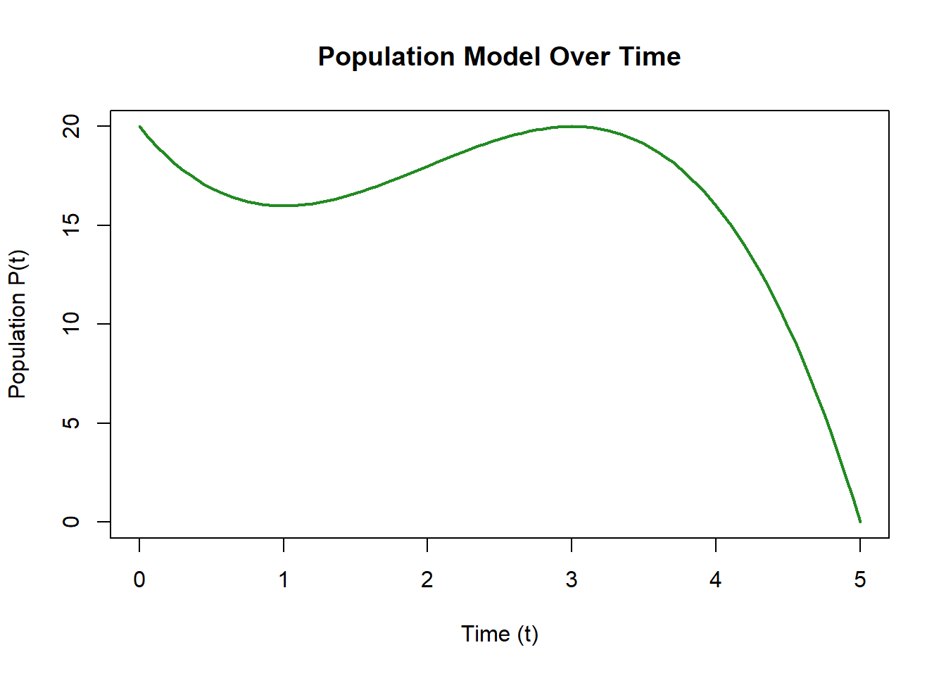
Figure 11.2: Graph of a population model over time showing how the population changes according to a cubic function.
Prompts
- Between which time intervals does the population increase or decrease?
- At what points might \(P'(t) = 0\)?
- Which point seems to be a local maximum and which a local minimum?
- How could this correspond to resource limitation or recovery in an ecosystem?
- What might happen if external factors (like drought or nutrient input) shifted these extrema?
11.2.7 Investigating the Derivative
Now that you’ve visualized the population curve, let’s explore how its rate of change behaves.
We’ll look at the derivative \(P'(t)\), which tells us whether the population is growing or shrinking at any moment.
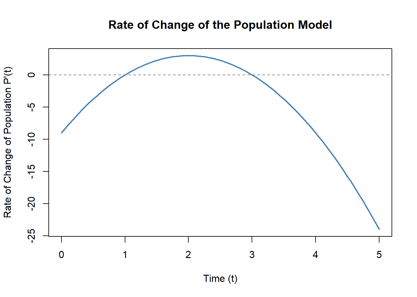
Figure 11.3: Graph of the derivative of the population model, showing how the rate of change of the population varies over time.
Prompts
- Where does \(P'(t) = 0\)?
- Between which values of \(t\) is \(P'(t)\) positive or negative?
- How does the sign of \(P'(t)\) relate to whether \(P(t)\) is increasing or decreasing?
- How do these intervals correspond to growth and decline phases in a population?
- What might cause these transitions in a real system (e.g., changes in food, space, or temperature)?
11.2.8 Linking Derivatives to System Behavior
Use your graph to fill in the table below.
| Observation | Derivative Sign | Population Behavior | Ecological Meaning |
|---|---|---|---|
| \(P'(t) > 0\) | Positive | \(P(t)\) increasing | Growth phase — population expanding |
| \(P'(t) = 0\) | Zero | Slope of \(P(t)\) flat | Turning point — possible max or min |
| \(P'(t) < 0\) | Negative | \(P(t)\) decreasing | Decline — competition or limitation |
11.2.9 Adding the Second Derivative
Next, explore the curvature of population change — whether the growth rate itself is speeding up or slowing down.
We’ll look at the second derivative \(P''(t)\).
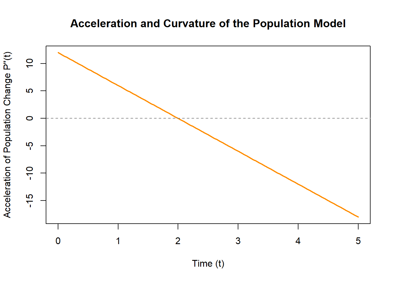
Figure 11.4: Graph of the second derivative of the population model, showing how the curvature and acceleration of population change vary over time.
Prompts
- Where does \(P''(t) = 0\)?
- What happens to \(P'(t)\) and \(P(t)\) near this point?
- How does the curvature (concavity) change before and after \(P''(t) = 0\)?
- What does a positive \(P''(t)\) tell you about the rate of change?
- What does a negative \(P''(t)\) indicate about slowing or reversing growth?
- In ecological terms, how might this point represent a tipping point or carrying capacity?
Now consider the second derivative, which describes how the rate of change itself is changing.
Use this table to connect the sign of \(P''(t)\) with system behavior.
| Observation | Second Derivative Sign | Curvature / Behavior of \(P(t)\) | Ecological Meaning |
|---|---|---|---|
| \(P''(t) > 0\) | Positive | Concave up — slope of \(P(t)\) increasing | Growth is accelerating; system recovering or resources increasing |
| \(P''(t) = 0\) | Zero | Point of inflection — curvature changes sign | Tipping point where growth shifts from accelerating to slowing |
| \(P''(t) < 0\) | Negative | Concave down — slope of \(P(t)\) decreasing | Growth is slowing; system approaching carrying capacity or limitation |
Discussion
- When \(P'(t) = 0\), what does this mean physically in the system?
- When \(P''(t) = 0\), what does this indicate about how the rate of change itself is behaving?
- How could identifying inflection points help forecast environmental transitions before they occur?
- Think of a real example — such as CO₂ uptake by vegetation, or lake temperature over a year.
- Where might you expect maxima, minima, and inflection points to occur?
- What could each tell you about system resilience or change?
- Where might you expect maxima, minima, and inflection points to occur?
Big Takeaway:
- \(f'(x)\) shows how fast something changes.
- \(f''(x)\) shows how that rate itself changes.
- Together, they reveal whether a system is accelerating, stabilizing, or reversing — the mathematical fingerprints of environmental balance.
11.3 Sign Chart Practice Worksheet
Goal: Practice creating first and second derivative sign charts for both original functions and their derivatives — learning to infer how a system behaves from either starting point.
Each part contains two examples:
- One starting from the original function \(f(x)\).
- One starting from the derivative \(f'(x)\).
11.3.1 Part 1 — Polynomial Patterns
A. Start from \(f(x)\)
Given
\[
f(x) = x^3 - 3x^2
\]
Solution
First compute derivatives.
\[
f'(x)=3x^2 - 6x = 3x(x-2),\qquad
f''(x)=6x - 6 = 6(x-1).
\]
For the first derivative sign chart, the critical points are \(x=0\) and \(x=2\).
Testing intervals:
- For \(x<0\), both factors are negative, so \(f'(x)>0\) and the function is increasing.
- For \(0<x<2\), the first factor is positive and the second is negative, so \(f'(x)<0\) and the function is decreasing.
- For \(x>2\), both factors are positive, so \(f'(x)>0\) and the function increases again.
Thus a local maximum occurs at \(x=0\) and a local minimum at \(x=2\).
For the second derivative, \(f''(x)=6(x-1)\), which changes sign at \(x=1\).
- For \(x<1\), \(f''(x)<0\): concave down.
- For \(x>1\), \(f''(x)>0\): concave up.
This marks an inflection point at \(x=1\).
Putting the information together:
The function rises to a local max at \(x=0\), falls to a local min at \(x=2\), and switches concavity at \(x=1\).
A sketch shows increasing → decreasing → increasing behavior, with concave down before \(x=1\) and concave up afterward.
B. Start from \(f'(x)\)
Given \[ f'(x)=2x(3-x) \]
Solution
Critical points occur at \(x=0\) and \(x=3\).
Testing signs:
- For \(x<0\), the first factor is negative, the second is positive, so \(f'(x)<0\): the function decreases.
- For \(0<x<3\), both factors are positive, so \(f'(x)>0\): the function increases.
- For \(x>3\), the first factor is positive and the second is negative, so \(f'(x)<0\): the function decreases.
This gives a local minimum at \(x=0\) and a local maximum at \(x=3\).
To analyze concavity, compute
\[
f'(x)=6x - 2x^2 \quad\Rightarrow\quad f''(x)=6 - 4x.
\]
The second derivative equals zero at \(x=1.5\).
- For \(x<1.5\), \(f''(x)>0\): concave up.
- For \(x>1.5\), \(f''(x)<0\): concave down.
Thus the function changes concavity at \(x=1.5\).
A sketch follows a decrease → increase → decrease pattern with concave up before \(1.5\) and concave down after.
11.3.2 Part 2 — Factored Derivatives and Flat Points (Corrected)
11.3.2.1 A. Start from \(f(x)\)
\[ f(x) = -x^3 + 3x^2 + 4x \]
Solution
✔️ Corrected Solution
1. First and second derivatives
\[ f'(x) = -3x^2 + 6x + 4 \]
\[ f''(x) = -6x + 6 = -6(x-1) \]
2. Critical points and monotonicity
Solve \(f'(x) = 0\):
\[ -3x^2 + 6x + 4 = 0 \]
\[ 3x^2 - 6x - 4 = 0 \]
\[ x = \frac{6 \pm \sqrt{36 + 48}}{6} = \frac{6 \pm \sqrt{84}}{6} = 1 \pm \frac{\sqrt{21}}{3} \]
So the critical points are:
\[ x_1 = 1 - \frac{\sqrt{21}}{3} \approx -0.53 \] \[ x_2 = 1 + \frac{\sqrt{21}}{3} \approx 2.53 \]
Sign of \(f'(x)\):
- \(x=-1\): \(f'(-1) = -5 < 0\) → decreasing
- \(x=0\): \(f'(0) = 4 > 0\) → increasing
- \(x=3\): \(f'(3) = -5 < 0\) → decreasing
Thus:
- Decreasing on \((-\infty,\;1-\tfrac{\sqrt{21}}{3})\)
- Increasing on \(\left(1-\tfrac{\sqrt{21}}{3},\;1+\tfrac{\sqrt{21}}{3}\right)\)
- Decreasing on \(\left(1+\tfrac{\sqrt{21}}{3},\;\infty\right)\)
Critical point classification:
- At \(x_1\): negative → positive ⇒ local minimum
- At \(x_2\): positive → negative ⇒ local maximum
3. Concavity and inflection point
\[ f''(x) = -6(x-1) \]
- If \(x < 1\): \(f''(x) > 0\) ⇒ concave up
- If \(x > 1\): \(f''(x) < 0\) ⇒ concave down
So:
- Concave up on \((-\infty, 1)\)
- Concave down on \((1, \infty)\)
Inflection point at:
\[ x = 1 \]
4. Overall behavior
- Decreasing → local minimum at \(x = 1 - \frac{\sqrt{21}}{3}\)
- Increasing → local maximum at \(x = 1 + \frac{\sqrt{21}}{3}\)
- Decreasing again
- Concave up for \(x<1\), concave down for \(x>1\), with an inflection at \(x=1\)
11.3.2.2 B. Start from \(f'(x)\)
\[ f'(x)= -3(x-1)(x+2)^2 \]
Solution
The derivative is zero at \(x=1\) and at \(x=-2\) (with multiplicity 2).
Because \((x+2)^2\) is always nonnegative and never changes sign, only the factor \((x-1)\) controls sign changes (and the leading \(-3\) flips everything).
Testing intervals:
- For \(x<-2\), \((x-1)<0\), the square is positive, and the leading \(-3\) makes the sign positive; the function increases.
- For \(-2<x<1\), \((x-1)<0\), sign remains the same, so the function now decreases.
- For \(x>1\), \((x-1)>0\), and the leading \(-3\) makes the product negative; the function continues decreasing.
Notably, the slope touches zero at \(x=-2\) but the sign does not change — a flat point, not an extremum.
A local maximum occurs at \(x=1\).
For concavity, differentiate: \[ f''(x)=-3\Big[(x+2)^2 + 2(x-1)(x+2)\Big] =-9x(x+2). \]
Concavity changes at \(x=0\) and \(x=-2\).
This gives multiple concavity regions and an inflection at \(x=0\); \(x=-2\) also behaves like an inflection but with a flat slope.
11.3.3 Part 3 — Exponential Behavior
11.3.3.1 A. Start from \(f(x)\)
\[ f(x)=e^x(x-2) \]
Solution
Compute derivatives: \[ f'(x)=e^x(x-1), \qquad f''(x)=e^x x. \]
For \(f'(x)\), the slope is zero at \(x=1\).
- For \(x<1\), the factor \((x-1)\) is negative → decreasing.
- For \(x>1\), the factor is positive → increasing.
Thus there is a local minimum at \(x=1\).
For the second derivative, \(f''(x)=e^x x\) changes sign at \(x=0\).
- For \(x<0\), negative → concave down.
- For \(x>0\), positive → concave up.
So inflection at \(x=0\).
Long-term behavior:
As \(x\to\infty\), the exponential dominates and \(f(x)\to\infty\).
As \(x\to-\infty\), the exponential goes to zero from the negative side, and \(f(x)\to 0^{-}\).
11.3.4 Part 4 — Undefined Derivatives and Asymptotes
11.3.4.1 A. Start from \(f(x)\)
\[ f(x)=\frac{x}{x-1} \]
Solution
Differentiate: \[ f'(x)= -\frac{1}{(x-1)^2},\qquad f''(x)=\frac{2}{(x-1)^3}. \]
The first derivative is never zero, so the function has no local maxima or minima.
It is always decreasing because the numerator is \(-1\) and the square in the denominator is always positive.
Both derivatives are undefined at \(x=1\), giving a vertical asymptote.
The second derivative changes sign at the asymptote:
- Left of 1, the denominator is negative → \(f''(x)<0\): concave down.
- Right of 1, the denominator is positive → \(f''(x)>0\): concave up.
The function approaches the horizontal asymptote \(y=1\) as \(x\to\pm\infty\).
11.3.4.2 B. Start from \(f'(x)\)
\[ f'(x)=\frac{e^x(x^2-4)}{x-2} \]
Solution
The derivative is zero when \(x^2-4=0\), so at \(x=-2\) and \(x=2\).
It is undefined at \(x=2\) because the denominator also becomes zero there.
Break the real line at \(-2\) and \(2\).
Testing intervals:
- For \(x<-2\), \(x^2-4>0\) and the denominator is negative, so the slope is negative: the function decreases.
- For \(-2<x<2\), \(x^2-4<0\) but the denominator is also negative, so slope is positive: the function increases.
- For \(x>2\), both numerator and denominator are positive, so slope is positive: the function continues increasing.
Thus there is a local minimum at \(x=-2\).
At \(x=2\), the derivative is undefined; this usually signals a vertical asymptote or sharp corner.
The function increases on both sides of \(x=2\).
11.3.5 Reflection — From Slopes to Shapes
Solution
Starting from \(f(x)\) means you compute everything from scratch; starting from \(f'(x)\) forces you to infer the function’s shape from slope information.
From \(f'(x)\) alone, you can determine where the function increases or decreases, where maxima and minima occur, and whether there might be asymptotes.
To know concavity or inflection points, though, you need \(f''(x)\).
In environmental contexts, maxima might represent carrying capacities or peak resources, minima might represent low points in population or nutrient availability, and inflection points often mark transitions such as switching from accelerating to slowing growth.
11.4 Challenge Problems — Sign Charts & Shape Analysis
Each problem includes three reveal options:
- Check 1st derivative
- Check 2nd derivative
- Full solution at the end password will be shared at the end of class
Challenge 2 — Rational Function With Two Asymptotes
\[ f(x)=\frac{1}{x^2 - 1} \]
Check 1st derivative
Differentiate using the chain rule:
\[ f'(x)=\frac{-2x}{(x^2 - 1)^2}. \]
Critical point comes from the numerator:
\[ -2x = 0 \quad\Longrightarrow\quad x = 0. \]
Derivative is undefined at:
\[ x = -1,\qquad x = 1 \]
These are vertical asymptotes.
Sign chart:
- Increasing on \((-\infty,-1)\) and \((-1,0)\)
- Decreasing on \((0,1)\) and \((1,\infty)\)
Thus the function has a local maximum at:
\[ f(0) = -1. \]
Check 2nd derivative
After simplification, the second derivative is:
\[ f''(x)=\frac{6x^2 + 2}{(x^2 - 1)^3}. \]
The numerator is always positive, so concavity is determined by the denominator.
Breakpoints for concavity:
- \(x = -1,\; x = 1\) (vertical asymptotes)
Test intervals:
| Interval | Sign of \(f''(x)\) | Concavity |
|---|---|---|
| \((-\infty, -1)\) | + | Concave up |
| \((-1, 1)\) | – | Concave down |
| \((1, \infty)\) | + | Concave up |
There is no inflection point, because concavity changes only across discontinuities.
Challenge 3 — Repeated Critical Point + Multiple Inflection Points
\[ f(x)=x^4 - 4x^3 \]
Check 1st derivative
Differentiate:
\[ f'(x)=4x^3 - 12x^2 = 4x^2(x - 3) \]
Critical points:
- \(x = 0\) (double root)
- \(x = 3\)
Sign pattern:
- For \(x < 3\): \(x-3 < 0\), and \(4x^2 \ge 0\) ⇒ \(f'(x) < 0\)
- For \(x > 3\): \(x-3 > 0\), \(f'(x) > 0\)
Thus:
- Decreasing on \((-\infty, 3)\)
- Increasing on \((3, \infty)\)
- At \(x = 0\), slope is zero but no sign change ⇒ a flat point, not an extremum
- At \(x = 3\), slope switches from − to + ⇒ local minimum
Check 2nd derivative
Differentiate again:
\[ f''(x)=12x^2 - 24x = 12x(x - 2) \]
Inflection points occur where \(f''(x)=0\):
\[ x = 0, \quad x = 2 \]
Concavity pattern (test the sign of \(f''\)):
- For \(x < 0\): both \(x\) and \(x-2\) negative ⇒ \(f''(x) > 0\) → concave up
- For \(0 < x < 2\): \(x > 0\) but \(x-2 < 0\) ⇒ \(f''(x) < 0\) → concave down
- For \(x > 2\): both factors positive ⇒ \(f''(x) > 0\) → concave up
So concavity transitions:
\[ \text{concave up} \;\to\; \text{concave down} \;\to\; \text{concave up} \]
with legitimate inflection points at \(x = 0\) and \(x = 2\).
Challenge 4 — Always Increasing, Multiple Inflection Points
\[ f(x)=\frac{e^{x}}{x^{2}+1} \]
NOTE: Factoring the second derivative is beyond the scope of this class so use this as the second derivative and its critical points to construct a sign chart.
Thus the real solutions of \(f''(x)=0\) occur at
\[ f''(x)= \frac{ e^{x}\left(x^{4}-4x^{3}+8x^{2}-4x-1\right) }{ (x^{2}+1)^{3} }. \]
\[ x \approx -0.18, \qquad x = 1. \]
Check 1st derivative
Differentiate:
\[ f'(x) = \frac{e^x(x^2+1) - e^x(2x)}{(x^2+1)^2} = \frac{e^x(x^2 - 2x + 1)}{(x^2+1)^2}. \]
Factor the numerator:
\[ f'(x)=\frac{e^x (x-1)^2}{(x^2+1)^2}. \]
All factors are nonnegative, and the derivative is zero only when \(x=1\).
The function is therefore increasing for all real \(x\), with a horizontal tangent at \(x=1\) but no local extremum there.
Check 2nd derivative
Differentiate \(f'(x)=e^x(x-1)^2(x^2+1)^{-2}\):
\[ f''(x)= \frac{ e^{x}\left(x^{4}-4x^{3}+8x^{2}-4x-1\right) }{ (x^{2}+1)^{3} }. \]
The denominator is always positive, so the sign depends on the numerator
\[
x^{4}-4x^{3}+8x^{2}-4x-1.
\]
Factoring shows it equals
\[
(x-1)\bigl(x^{3}-3x^{2}+5x+1\bigr).
\]
Thus the real solutions of \(f''(x)=0\) occur at
\[ x \approx -0.18, \qquad x = 1. \]
Testing each interval gives the concavity pattern:
- up on \((-\infty,\; -0.18)\)
- down on \((-0.18,\; 1)\)
- up on \((1,\; \infty)\)
So the function has two inflection points and remains always increasing.
Challenge 5 — A Function With an S-Shaped Curve
Consider the function
\[
f(x)=\frac{50}{1+2e^{-x}}.
\]
- Compute \(f'(x)\) and \(f''(x)\).
- Determine intervals of increase/decrease and concavity.
- Identify any critical points and inflection points.
- Check the long-term limits:
- What happens to \(f(x)\) as \(x\to -\infty\)?
- What happens to \(f(x)\) as \(x\to +\infty\)?
- What happens to \(f(x)\) as \(x\to -\infty\)?
- Sketch the curve and label the important features.
- Have you seen an equation with this structure in any of your other classes?
Check 1st derivative
Rewrite the function as
\[
f(x)=50(1+2e^{-x})^{-1}.
\]
Differentiate: \[ f'(x)=50\cdot(-1)(1+2e^{-x})^{-2}\cdot(2e^{-x}\cdot -1) =\frac{100e^{-x}}{(1+2e^{-x})^2}. \]
Rewriting using \(e^x\): \[ f'(x)=\frac{100e^{x}}{(e^{x}+2)^2}. \]
All factors are positive, so \(f'(x)>0\) for every real \(x\).
The function is increasing everywhere.
Check 2nd derivative
Differentiating using the form
\[
f'(x)=\frac{100e^{x}}{(e^{x}+2)^2}
\]
gives, after simplification:
\[ f''(x)=\frac{100e^{x}(2 - e^{x})}{(e^{x}+2)^3}. \]
The denominator is positive for all \(x\).
Thus the sign comes from \((2 - e^{x})\):
- For \(x < \ln 2\): \(e^{x}<2\) and \(f''(x)>0\), so the graph is concave up.
- For \(x > \ln 2\): \(e^{x}>2\) and \(f''(x)<0\), so the graph is concave down.
There is an inflection point at
\[
x = \ln 2.
\]
11.4.1 Solution to Challenge Problems
Full Challenge Solutions
CHALLEGE 1 Solution
Start with: \[ f'(x) = 2xe^{-x} + (x^2 - 4)(-e^{-x}) = e^{-x}(-x^2 + 2x + 4). \]
Since \(e^{-x} > 0\), the sign of the derivative is controlled by
\(-x^2 + 2x + 4\), which has roots
\[ x = 1 - \sqrt5 \approx -1.236, \qquad x = 1 + \sqrt5 \approx 3.236. \]
Sign analysis:
- Decreasing on \((-\infty, 1 - \sqrt5)\)
- Increasing on \((1 - \sqrt5,\; 1 + \sqrt5)\)
- Decreasing on \((1 + \sqrt5, \infty)\)
Thus:
- Local maximum at \(x = 1 - \sqrt5\)
- Local minimum at \(x = 1 + \sqrt5\)
Next, \[ f''(x)= e^{-x}(x^2 - 4x - 2). \]
The quadratic has roots: \[ x = 2 - \sqrt6 \approx -0.449, \qquad x = 2 + \sqrt6 \approx 4.449. \]
Because the quadratic opens upward, the concavity pattern is:
- Concave up for \(x < 2 - \sqrt6\)
- Concave down for \(2 - \sqrt6 < x < 2 + \sqrt6\)
- Concave up for \(x > 2 + \sqrt6\)
Thus the function has two inflection points, one on each side of where the exponential begins to dominate.
The complete shape:
- Decreasing → increasing → decreasing
- Inflection → concave down → inflection
- Exponential factor affects magnitude but not sign behavior
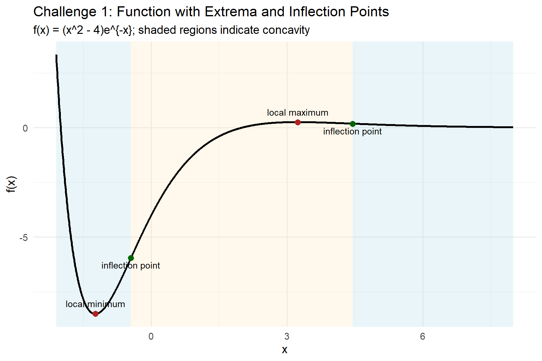
Figure 11.5: Graph of the function f(x) = (x^2 - 4)e^{-x} with local extrema, inflection points, and shaded intervals showing where the graph is concave up or concave down.
CHALLEGE 2 Solution
1. First derivative analysis
\[ f'(x)=\frac{-2x}{(x^2 - 1)^2} \]
Critical point: \[ x = 0. \]
Increasing on: \[ (-\infty,-1),\qquad (-1,0) \]
Decreasing on: \[ (0,1),\qquad (1,\infty) \]
So the function has a local maximum at: \[ f(0) = -1. \]
2. Asymptote analysis (limits)
The function is undefined at: \[ x=-1,\qquad x=1 \]
Asymptote at \(x=-1\)
\[ \lim_{x\to -1^-} f(x) = +\infty, \qquad \lim_{x\to -1^+} f(x) = -\infty \]
So \(x=-1\) is a vertical asymptote.
Asymptote at \(x=1\)
\[ \lim_{x\to 1^-} f(x) = -\infty, \qquad \lim_{x\to 1^+} f(x) = +\infty \]
So \(x=1\) is also a vertical asymptote.
3. Second derivative and concavity
\[ f''(x)=\frac{6x^2 + 2}{(x^2 - 1)^3} \]
The numerator \(6x^2+2\) is always positive, so concavity is determined entirely by the denominator.
Concavity pattern: - Concave up on \((-\infty,-1)\) - Concave down on \((-1,1)\) - Concave up on \((1,\infty)\)
There are no inflection points, because the concavity change occurs at vertical asymptotes.
4. Complete shape
- One critical point → local max at \(x=0\)
- Vertical asymptotes at \(x=-1\) and \(x=1\)
- Concavity: up → down → up
- Function breaks naturally into three separate branches
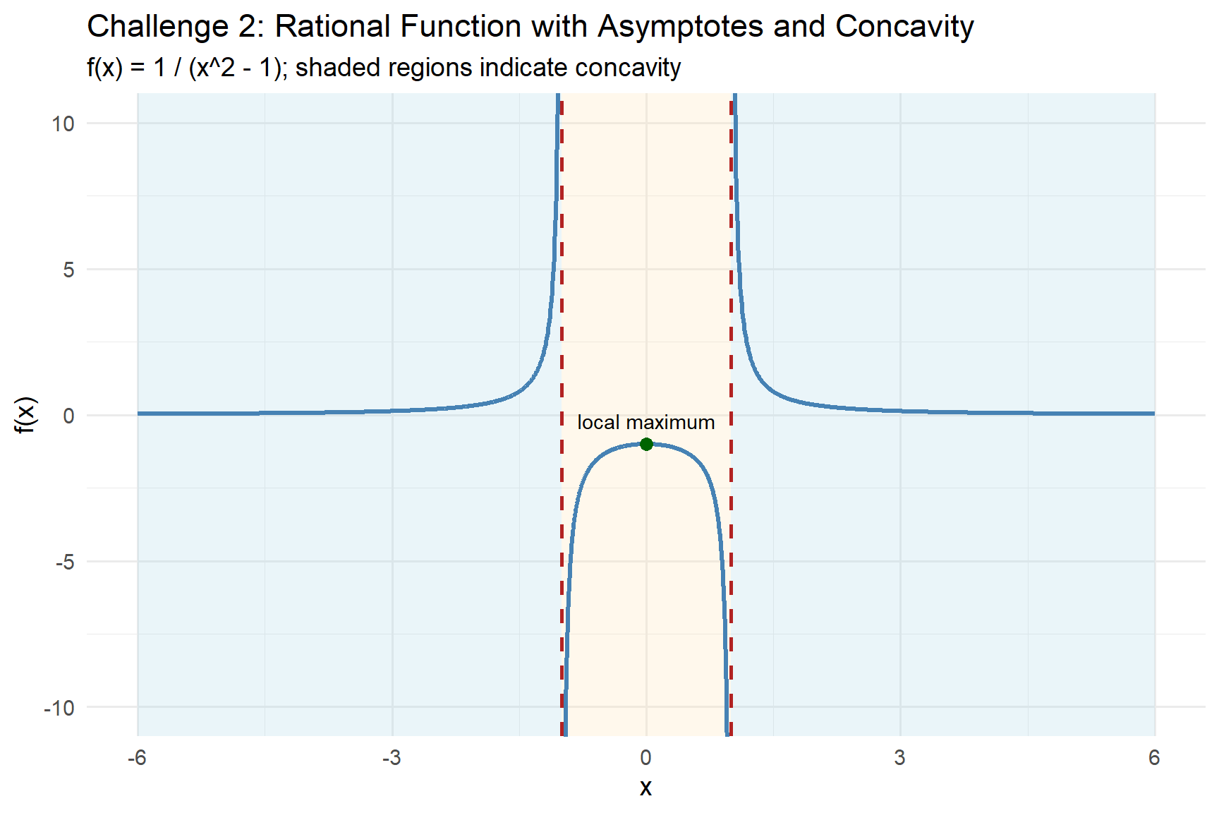
Figure 11.6: Graph of the rational function f(x) = 1/(x^2 - 1) showing its local maximum, vertical asymptotes, and intervals of concavity.
CHALLEGE 3 Solution
1. First derivative and monotonicity
\[ f'(x)=4x^2(x - 3) \]
Zeros at:
- \(x = 0\) (double root → slope flattens but does not change sign)
- \(x = 3\) (simple root → sign change)
Sign pattern:
- \(f'(x) < 0\) for all \(x < 3\)
- \(f'(x) > 0\) for all \(x > 3\)
Thus:
- Always decreasing before \(x = 3\)
- Always increasing after \(x = 3\)
- A local minimum at \(x = 3\)
- A flat point but no extremum at \(x = 0\)
2. Concavity (second derivative)
\[ f''(x) = 12x(x - 2) \]
Set second derivative = 0:
- \(x = 0\)
- \(x = 2\)
Concavity pattern:
- Concave up for \(x < 0\)
- Concave down for \(0 < x < 2\)
- Concave up for \(x > 2\)
Thus there are two inflection points:
\[ x = 0, \qquad x = 2 \]
3. Overall behavior and sketch description
- The function decreases steadily until \(x = 3\), where it achieves a local minimum.
- After \(x = 3\), it increases forever.
- Concavity:
- Up before 0
- Down between 0 and 2
- Up after 2
- Up before 0
- Inflection points at \(x = 0\) and \(x = 2\).
- The point \(x = 0\) is especially interesting: the slope is zero there but the graph is still decreasing.
This gives the characteristic “flatten → dip → rise” shape typical of a quartic with asymmetric coefficients.
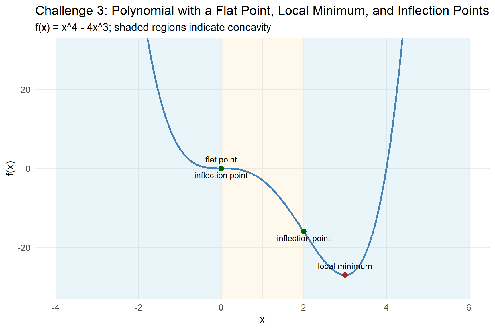
Figure 11.7: Graph of the polynomial function f(x) = x^4 - 4x^3 showing a flat critical point, a local minimum, inflection points, and shaded intervals of concavity.
CHALLEGE 4 Solution
The first derivative is
\[ f'(x)=\frac{e^x (x-1)^2}{(x^2+1)^2}, \]
which is never negative and equals zero only at \(x=1\).
Thus the function is increasing everywhere, with a horizontal tangent at \(x=1\) but no local maximum or minimum.
For concavity, the correct second derivative is
\[ f''(x)= \frac{ e^{x}\left(x^{4}-4x^{3}+8x^{2}-4x-1\right) }{ (x^{2}+1)^{3} }, \]
and the sign depends on the numerator
\[ x^{4}-4x^{3}+8x^{2}-4x-1 = (x-1)\bigl(x^{3}-3x^{2}+5x+1\bigr). \]
The cubic has one real root (the other two are complex), located at
\[ x \approx -0.18, \]
along with the linear-factor root at \(x=1\).
These give the two real inflection points of the function.
Testing each interval shows the concavity pattern:
- concave up on \((-\infty,\,-0.18)\)
- concave down on \((-0.18,\;1)\)
- concave up on \((1,\;\infty)\)
Summary:
The function rises smoothly for all \(x\), flattens at \(x=1\) without forming an extremum, and changes concavity twice, creating two inflection points while remaining always increasing.
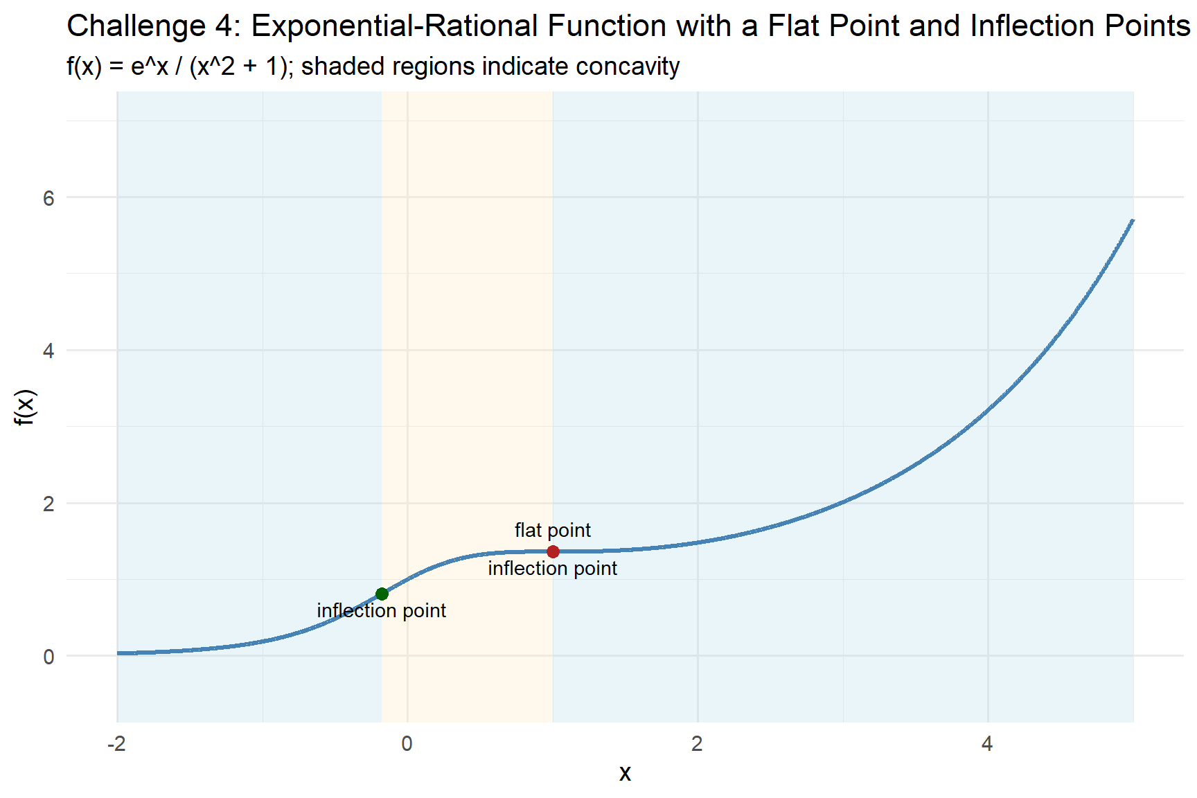
Figure 11.8: Graph of the function f(x) = e^x / (x^2 + 1) showing inflection points, a flat point, and shaded intervals of concavity.
CHALLEGE 5 Solution
The derivative
\[
f'(x)=\frac{100e^{x}}{(e^{x}+2)^2}
\]
is positive for all real \(x\), so the function has no local maxima or minima and increases steadily for all inputs.
The second derivative
\[
f''(x)=\frac{100e^{x}(2 - e^{x})}{(e^{x}+2)^3}
\]
changes sign when \(e^{x}=2\).
This occurs at \(x=\ln 2\), which is an inflection point.
The concavity structure is:
- concave up for \(x<\ln 2\)
- concave down for \(x>\ln 2\)
For the long-term limits:
As \(x\to -\infty\), \(e^{-x}\to\infty\), so the denominator \(1+2e^{-x}\) becomes very large and
\[
\lim_{x\to -\infty} f(x)=0.
\]
As \(x\to +\infty\), \(e^{-x}\to 0\), so the denominator approaches \(1\) and
\[
\lim_{x\to +\infty} f(x)=50.
\]
The resulting graph has a smooth S-shape, increases for all \(x\), and levels off near these two horizontal limits.
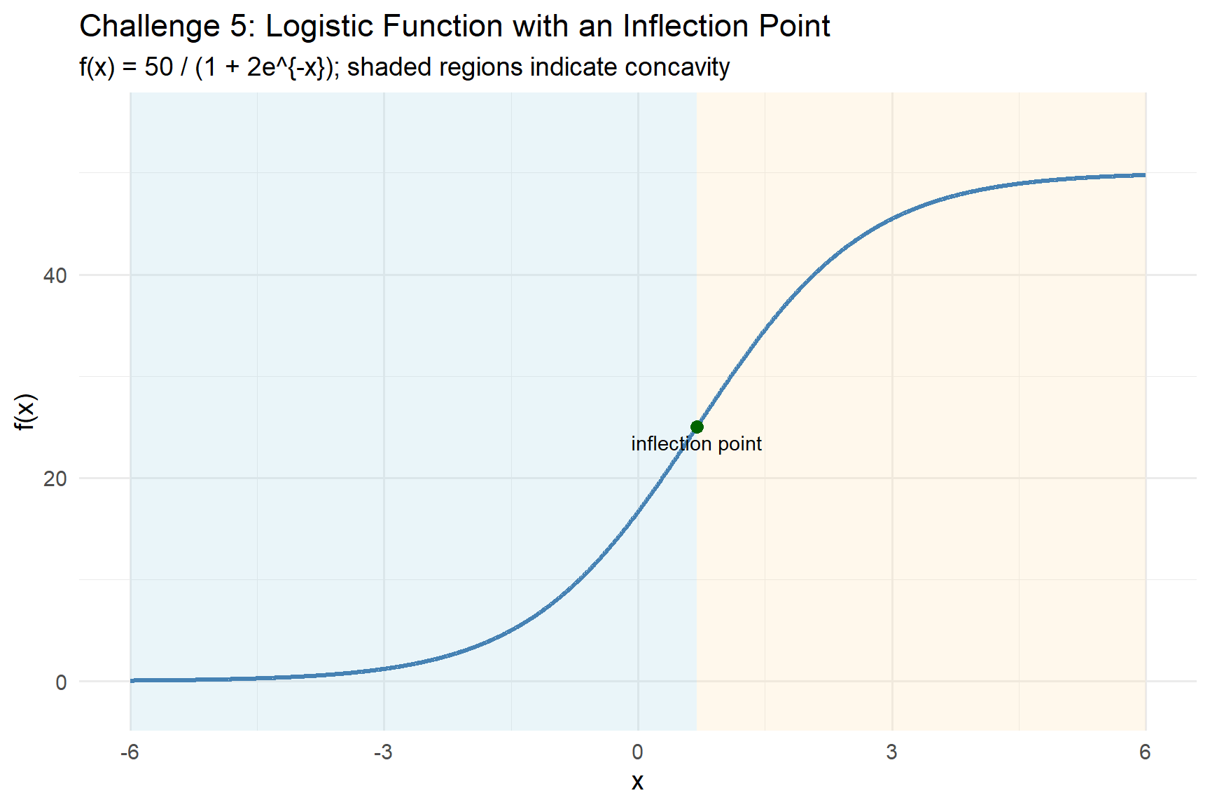
Figure 11.9: Graph of the function f(x) = 50 / (1 + 2e^{-x}) showing its S-shaped growth, inflection point, and shaded intervals of concavity.