Chapter 14 Student Discussion + Activity Template: Applications of Integration

Goal for this section
Build the habit of asking: What is accumulating? Over what variable? What do the units imply?
Then practice translating that story into an integral, and interpreting the result.

---

14.1 Discussion Prompts (use as think–pair–share)

Prompt Set A: What is an integral doing? (meaning first)

1. In your own words, what does “accumulation” mean? Give one real-world example that is not about area.
2. What’s the difference between a rate and a total? Give an example of each.
3. Why does “small pieces add up” naturally lead to an integral?
4. What does the \(dx\) or \(dt\) tell you about what you are adding up?
5. What would it mean if an integral gave a negative answer in a real system?

Prompt Set B: Units as a reality check

6. Suppose \(r(t)\) has units of mm/hr and you integrate \(r(t)\,dt\). What are the units of the result? Does that match what you want to measure?
7. Suppose \(\rho(x,y)\) has units of kg/m\(^2\). What does \(\iint_R \rho(x,y)\,dA\) represent?
8. If your units don’t cancel cleanly into something meaningful, what are two possible reasons?

Prompt Set C: Total vs net vs “area between curves”

9. Compare these three questions. Which one matches each integral, and why?
   • 1. “How much was produced?”
   • 2. “What was the net change?”
   • 3. “How different are these two curves overall?” \[ \int_0^T P(t)\,dt,\qquad \int_0^T (P(t)-L(t))\,dt,\qquad \int_0^T |P(t)-L(t)|\,dt \]
10. If two curves cross, what changes about the setup for geometric area? What doesn’t change for net accumulation?

Prompt Set D: When data are messy (numerical integration)

11. When you measure something daily, why isn’t the “true integral” immediately available?
12. What do you gain by fitting a smooth function to data? What might you lose?
13. In your streamflow example, why were the “fit” total and the “rectangles” total close but not identical?
14. If you were writing a report, when would you trust the fitted model more than the data rectangles? When would you do the opposite?

---

14.2 In-Class Mini-Workflow

Step 1: Story - What is changing?
- What is being added up?
- Over what variable?

Step 2: Units - Write the units of the integrand. - Write the units of the differential (\(dx\), \(dt\), \(dA\), \(dV\)). - Multiply them to predict the units of the result.

Step 3: Setup - Total? Net? Area between curves? Average? - Write the correct integral.

Step 4: Compute or approximate - If there’s a clean function, integrate. - If data are discrete or messy, approximate numerically.

Step 5: Interpret - What does the number mean in context? - Sense check: Is the sign reasonable? Is the magnitude plausible?

---

14.3 Worked Example 1: Average Value

Task
Compute the average value of \[ f(x)=x^2 \] on \([2,4]\), and interpret it as an “equal-area rectangle.”

Prompts during the solution

• What does “average value” mean for a function?
• Why are we dividing by \(b-a\)?
• What does the rectangle represent geometrically?

Solution skeleton General form of the average equation

\[ f_{\text{avg}}=\frac{1}{b-a}\int_a^b f(x)\,dx \]

So in this example:

\[ f_{\text{avg}}=\frac{1}{4-2}\int_2^4 x^2\,dx \] \[ \int_2^4 x^2\,dx = \left.\frac{x^3}{3}\right|_2^4 \] \[ f_{\text{avg}}=\frac{1}{2}\cdot \frac{56}{3}=\frac{28}{3} \]

Follow-up prompt

• If \(f(x)\) were sometimes negative, how would that affect the “average”?

---

14.4 Worked Example 2: Area Between Curves with a Crossing

Task
Find the geometric area between \[ f(x)=x,\qquad g(x)=x^3 \] on \([-1,1]\).

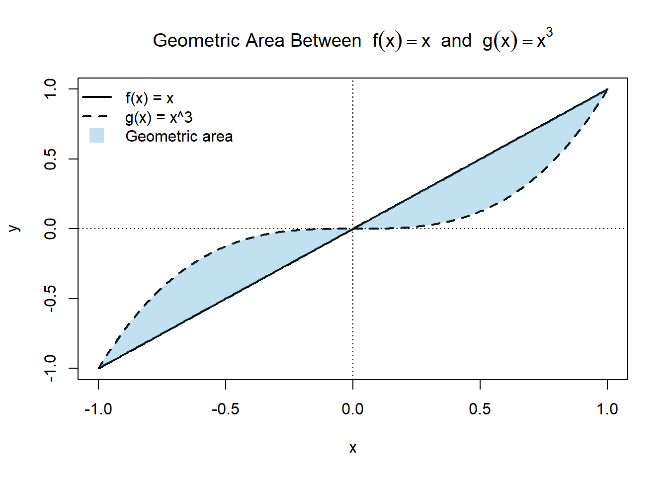
Student prompts

1. Where do the curves intersect?
2. On \([-1,0]\), which is on top?
3. On \([0,1]\), which is on top?
4. Why can’t we just do \(\int_{-1}^{1} (f-g)\,dx\) and call that “area”?

Solution skeleton

• Intersections: \(x=-1,0,1\)
• Set up: \[ \text{Area}=\int_{-1}^{0} (g-f)\,dx + \int_{0}^{1} (f-g)\,dx \]
• Compute and add.

Extension

• Replace “area” with “net difference.” What changes in the setup?

---

14.5 Worked Example 3: Numerical Integration from Data (no curve fitting)

Task
You measured daily streamflow \(Q_i\) (m\(^3\)/s) for 7 days. Estimate the total volume of water that passed the gauge in that week.

Give students a small dataset

Day: 1 2 3 4 5 6 7
\(Q\): 42 55 61 58 49 45 40 (m\(^3\)/s)

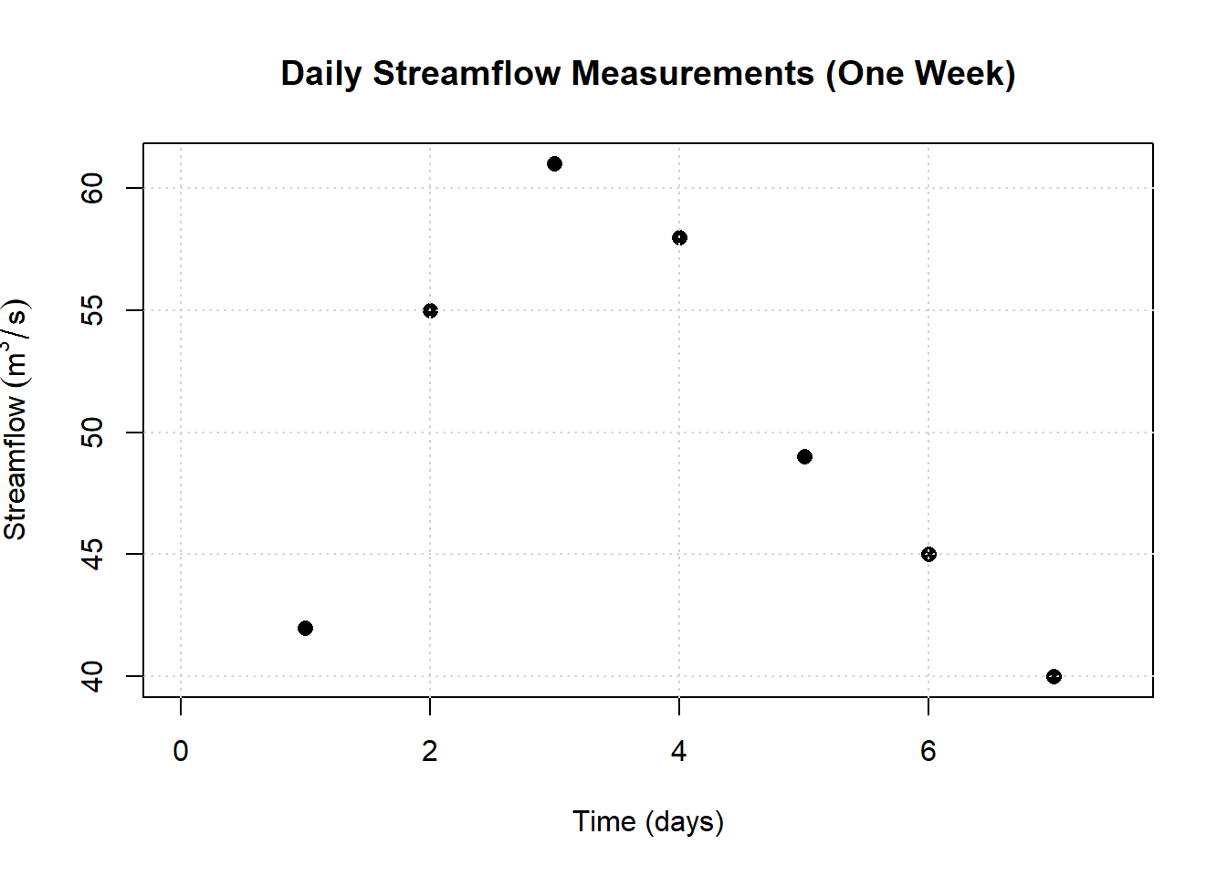
Prompts

1. If each value is “m\(^3\)/s,” what does multiplying by one day do to the units?
2. Why do we need to convert days to seconds?
3. Use rectangles to estimate weekly volume: \[ V \approx \sum_{i=1}^{7} Q_i \,\Delta t \]
4. If you used trapezoids instead, would the estimate increase or decrease? Why?

Solution skeleton

• \(\Delta t = 86400\) s per day
• Rectangles: \[ V \approx 86400\sum_{i=1}^{7} Q_i \]
• (Optional) trapezoids for comparison: \[ V \approx \frac{86400}{2}\left(Q_1+2Q_2+\cdots+2Q_6+Q_7\right) \]

Reflection prompt

• Which method (rectangles or trapezoids) seems more defensible here, and why?

---

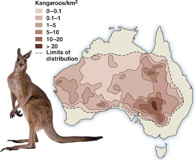
14.6 Counting Species

How would you work out how many trees there are in a forest? Or how many whales in the ocean?

Come up with a method for working out how many trees there are on this campus?

How would I work out how many Kangaroos there are in Australia?

14.7 Thinking with Double Integrals

Purpose of this activity
Practice translating spatial accumulation stories into double integrals, before worrying about heavy computation. The focus is on:

• identifying what is accumulating,
• understanding the region of integration,
• interpreting the result using units.

---

14.8 Part A: Conceptual Warm-Up (Think → Pair → Share)

Prompt 1: What is being accumulated?
For each statement below, decide whether a double integral is appropriate and explain why.

1. Total rainfall over a rectangular field during a storm.
   
2. Average air temperature along a hiking trail.
   
3. Total mass of algae in a shallow lake, where concentration varies by location.
   
4. Total distance traveled by a migrating animal.

---

Prompt 2: Units check

Suppose \(f(x,y)\) has units of kg/m².

1. What are the units of \(f(x,y)\,dA\)?
   
2. What are the units of \(\iint_R f(x,y)\,dA\)?
   
3. What real-world quantity might this integral represent?

---

14.9 Part B: From Single to Double Integrals

Prompt 3: Extending what you know

Recall: \[ \int_a^b f(x)\,dx \]

1. What does this accumulate?
2. What does the “small piece” look like?

Now compare with: \[ \iint_R f(x,y)\,dA \]

3. What is the small piece now?
4. How is the logic the same? How is it different?

---

14.10 Part C: Setting Up (Not Solving) Double Integrals

14.10.1 Example 1: Constant Density Over a Region

Suppose pollution is distributed uniformly over a rectangular area.

• Density: \(\rho(x,y) = 5\) kg/m²
  
• Region:
  \[ R = \{(x,y)\mid 0 \le x \le 4,\; 0 \le y \le 3\} \]

Student tasks

1. Write a double integral that represents the total pollutant mass.
2. Before computing anything, predict whether the answer should be:
   • small or large?
   • positive or zero?

Setup \[ \iint_R 5\,dA = \int_0^4 \int_0^3 5\,dy\,dx \]

Discussion prompt
Why does this integral reduce to “density × area”?

---

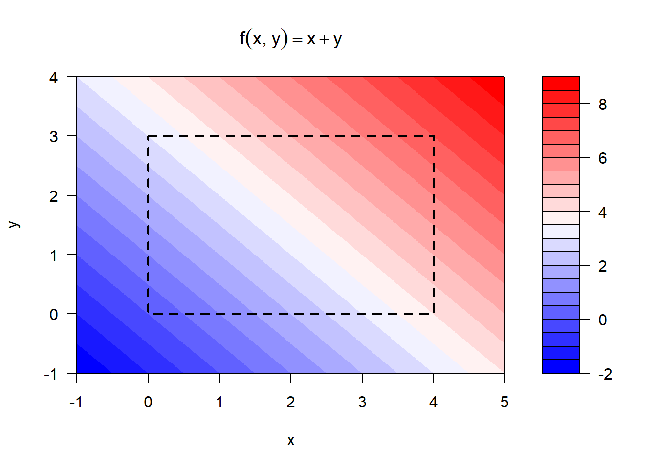
14.10.2 Example 2: Variable Density Over a Rectangle

Now suppose density varies with position: \[ \rho(x,y) = x + y \]

on the same region \[ R = \{(x,y)\mid 0 \le x \le 4,\; 0 \le y \le 3\}. \]

Student tasks

1. Write the double integral for total mass.
2. Decide whether it makes more sense to integrate with respect to \(x\) or \(y\) first.
3. What does “holding one variable constant” mean physically?

Setup \[ \iint_R (x+y)\,dA = \int_0^4 \int_0^3 (x+y)\,dy\,dx \]

(Do not compute yet — focus on interpretation.)

---

14.11 Part D: Interpreting Inner Integrals

Prompt 4: What does the inner integral represent?

Given: \[ \int_0^4 \left[\int_0^3 (x+y)\,dy\right] dx \]

1. What does the inner integral compute when \(x\) is fixed?
2. What does the outer integral add up?
3. How is this like “stacking” single integrals?

---

14.12 Part E: Symmetry and Cancellation

14.12.1 Example 3: When Things Cancel

Let \[ f(x,y) = y \] over the symmetric region \[ R = \{(x,y)\mid -2 \le x \le 2,\; -3 \le y \le 3\}. \]

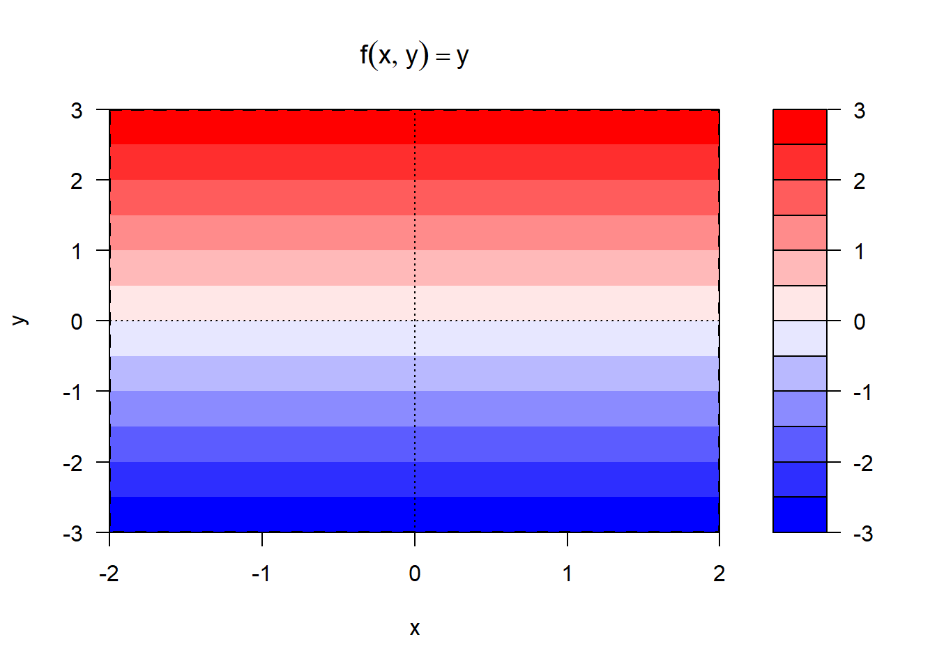
Student tasks

1. Sketch the region.
2. Predict the value of \[ \iint_R y\,dA \] before computing.
3. Explain your reasoning using symmetry.

Key idea prompt
What does it mean for a function to be “odd” in one variable over symmetric bounds?

---

14.13 Part F: Average Value Over a Region

Prompt 5: Average vs total

For a function \(f(x,y)\) over a region \(R\):

1. What does \(\iint_R f(x,y)\,dA\) represent?
2. How would you turn that into an average value over the region?

Definition \[ f_{\text{avg}} = \frac{1}{\text{Area}(R)} \iint_R f(x,y)\,dA \]

Think-pair-share

• What would the units of \(f_{\text{avg}}\) be?
• How does this mirror the 1D average value formula?

---

14.14 Area Between Two Curves — Conceptual and Computational Practice

These problems are designed to help you practice:

• Setting up top minus bottom
• Understanding what happens when curves cross
• Distinguishing net accumulation from geometric area
• Handling situations where functions are negative
• Interpreting integrals of rates

---

Problem 1 — Basic Geometric Area (No Crossing)

Consider
\[ f(x) = 6 - x^2 \]
\[ g(x) = 2 \]

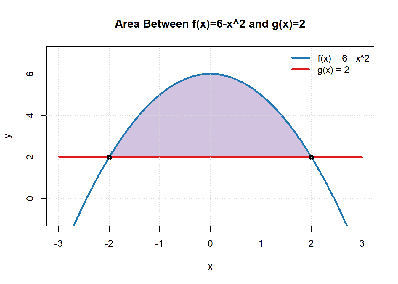
1. Find the points where the curves intersect.
2. Determine which function is on top between those points.
3. Set up the integral for the geometric area between the curves.
4. Evaluate the area.

---

Problem 2 — When Curves Cross

Consider
\[ f(x) = x \]
\[ g(x) = x^3 \]

on the interval \([-1,1]\).

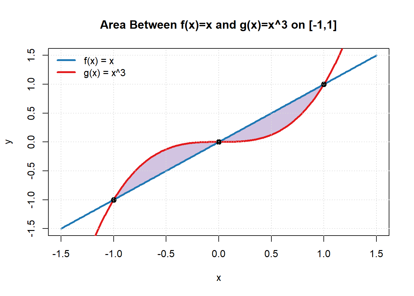
Part A — Intersection Points

1. Find all values of \(x\) where the functions are equal.
2. Determine which function is on top on each part of the interval.

Part B — Do NOT Split the Integral

Without breaking the interval apart, compute:

\[ \int_{-1}^{1} \big(f(x) - g(x)\big)\,dx \]

1. Evaluate the integral.
2. What does this value represent?
3. Why does cancellation occur?

Part C — Now Compute the Geometric Area

1. Identify where the functions switch which one is on top.
2. Split the integral at the intersection point(s).
3. Set up integrals that always compute top minus bottom.
4. Evaluate the total geometric area between the curves.

Part D — Reflection

1. Compare the answers from Parts B and C.
2. Why are they different?
3. When must an integral be split?
4. What does the unsplit integral actually measure?

---

Problem 3 — Net Change Between Two Rates

A lake has:

• Inflow rate: \[ I(t) = 5 + 2t \]

• Outflow rate: \[ O(t) = 3 + t \]

where \(t\) is in days and rates are in millions of gallons per day.

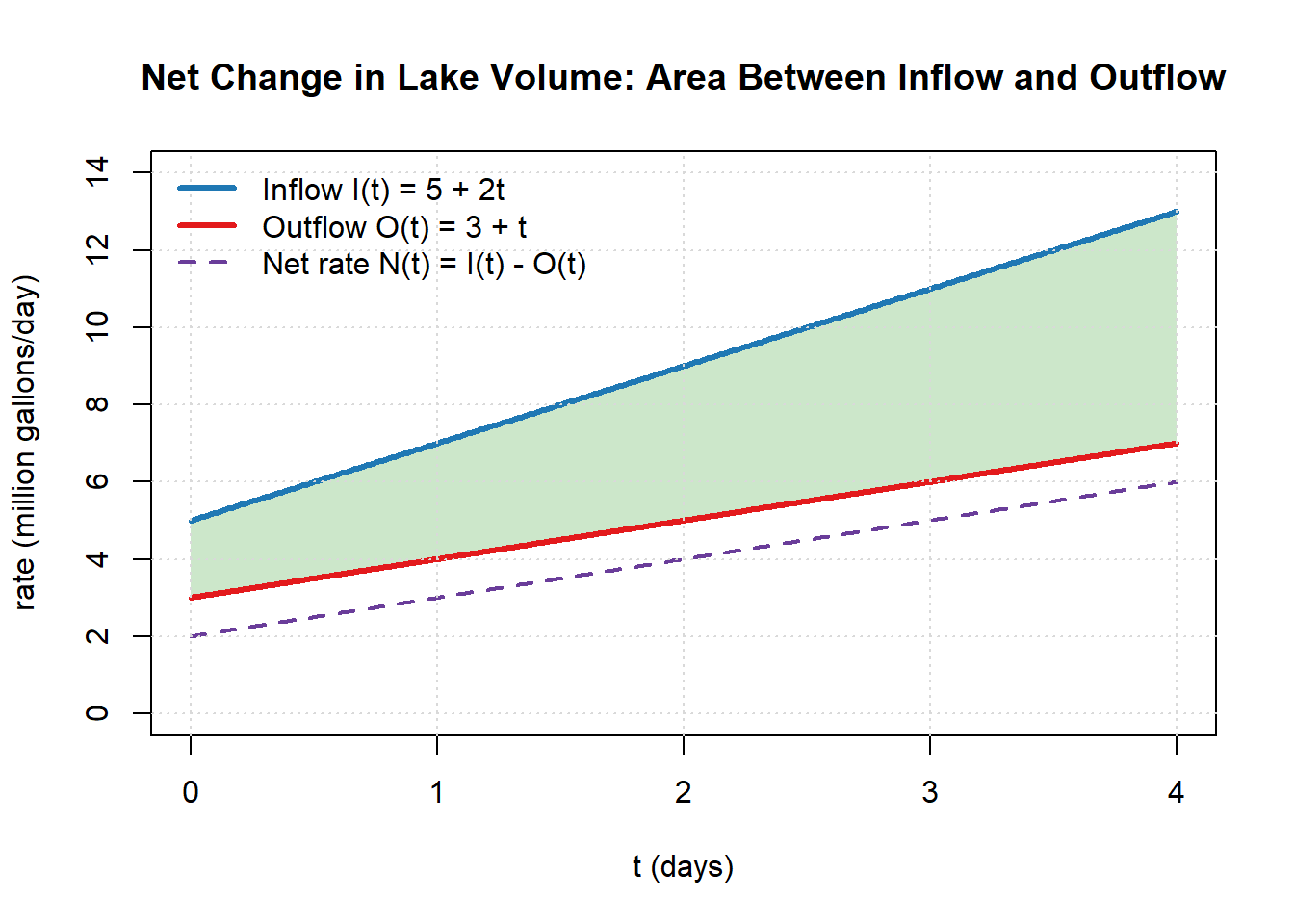
1. Write an expression for the net rate of change of the lake volume.
2. Over \(0 \le t \le 4\), compute the net change in water volume.
3. Does the lake gain or lose water overall?
4. Explain how this problem is structurally similar to area between curves.

---

Problem 4 — Crossing Rates (Net vs Geometric Difference)

Before working this problem, it is important to clarify what we mean by advantage.

At any single moment in time, each species has a growth rate. A growth rate tells us how fast the population is increasing at that instant. If one species has a larger growth rate than the other at time \(t\), then it is growing faster at that moment.

So we define the instantaneous advantage of Species 1 over Species 2 as

\[ R_1(t) - R_2(t). \]

• If this quantity is positive, Species 1 is growing faster.
• If it is negative, Species 2 is growing faster.
• If it is zero, neither species has an advantage at that moment.

But we are often interested in more than a snapshot. We may want to know:

• Which species gained more total growth over a time period?
• Did one species’ early advantage outweigh the other’s later advantage?

To answer that, we integrate.

\[ \int_a^b \big(R_1(t) - R_2(t)\big)\,dt \]

This integral represents the net advantage over the interval \([a,b]\).
Geometrically, it is the signed area between the two rate curves.

If positive and negative regions cancel, the net advantage may be zero — even though one species led for part of the time. If we instead integrate the absolute value,

\[ \int_a^b \left|R_1(t) - R_2(t)\right| dt, \]

we measure the total geometric difference, which captures how much the species differed overall, regardless of who was ahead.

Keep this distinction in mind as you work the problem below.

Two species have population growth rates:

\[ R_1(t) = 8 - t \]
\[ R_2(t) = t \]

for \(0 \le t \le 8\).

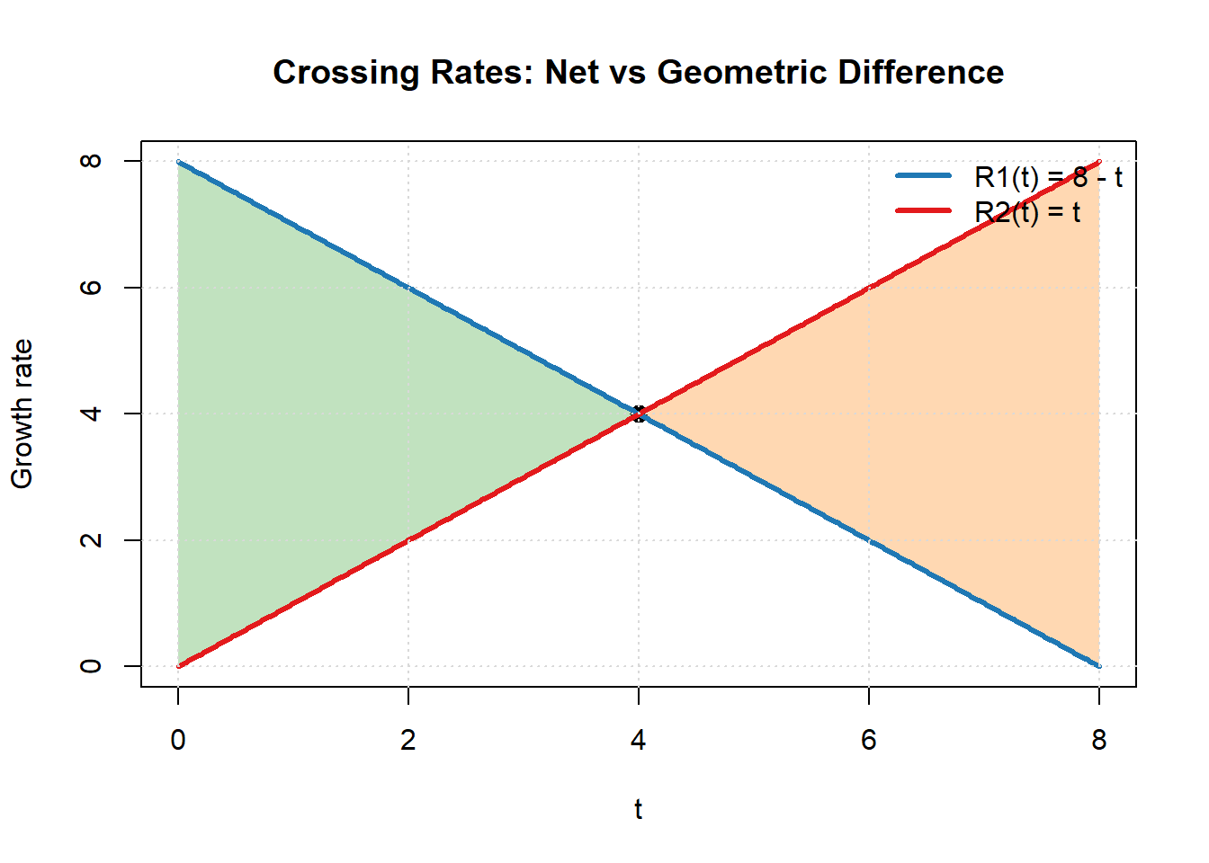
1. Find when the two rates are equal.
2. Compute the net advantage of Species 1 over Species 2 on \([0,8]\) using a single integral.
3. Interpret your result.
4. Now compute the total geometric difference between the rates on the interval.
5. Why are the two answers different?

---

Problem 5 — Both Functions Negative

Consider
\[ f(x) = -x^2 - 1 \]
\[ g(x) = -3 \]

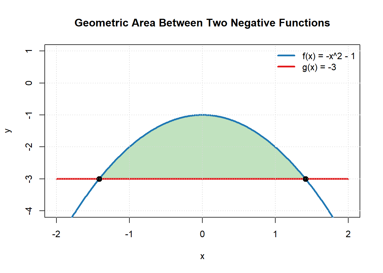
1. Find the intersection points.
2. Determine which function is on top between those points.
3. Set up the integral for the geometric area between the curves.
4. Evaluate the area.
5. Explain why the result is positive even though both functions are negative.
6. What would happen if you accidentally reversed top and bottom?

---

Core Ideas to Understand

• Area between curves is always top minus bottom.
• When curves cross, you must consider where the sign changes.
• A single integral measures net accumulation, not always geometric area.
• Cancellation reflects signed area.
• Negative functions do not break the method — subtraction handles the sign.

Click to Unlock Solutions

14.15 Double and Triple Integrals — Conceptual and Computational Practice

These problems are designed to help you practice:

• Setting up double and triple integrals from geometric descriptions
  
• Interpreting accumulation over area and volume
  
• Distinguishing net accumulation from total magnitude
  
• Correctly identifying bounds of integration
  
• Understanding when symmetry simplifies computation

---

Problem 1 — Volume Under a Surface (Basic Double Integral)

Let \[ f(x,y) = 4 - x - y \]

over the rectangular region \[ R = \{(x,y) \mid 0 \le x \le 2,\; 0 \le y \le 1\}. \]

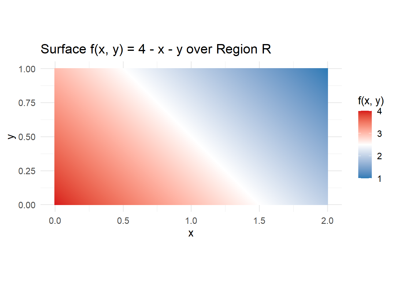
1. Write the double integral that represents the volume under the surface.
   
2. Evaluate the integral.
   
3. Explain why this integral represents volume.
   

---

Problem 2 — Net Accumulation Over a Region (Sign Matters)

Suppose a pollutant concentration over a square lake is modeled by \[ C(x,y) = x - y \]

over the square \[ 0 \le x \le 2,\quad 0 \le y \le 2. \]

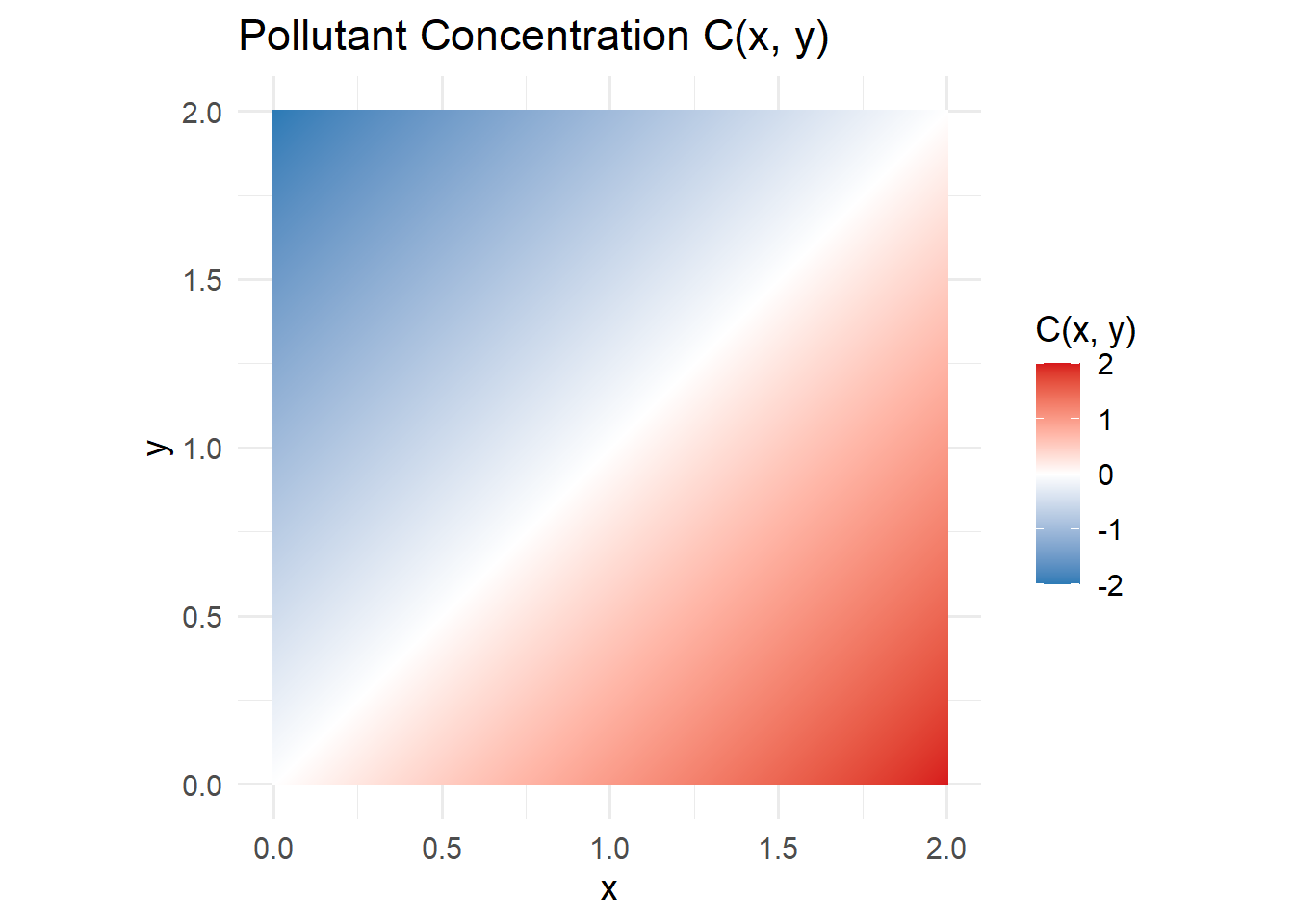::: promptbox 1. Set up the double integral representing the total (net) pollutant mass.
2. Evaluate the integral without splitting the region.
3. Why does cancellation occur?
4. Does this mean there is no pollutant present? Explain.
:::

---

Problem 3 — Curved Boundary and Sign Change

Let \[ f(x,y) = x^2 - y \]

over the region bounded by \[ y = 0, \quad y = x^2, \quad 0 \le x \le 2. \]

Hint: set up your integral with dy being the interior integral

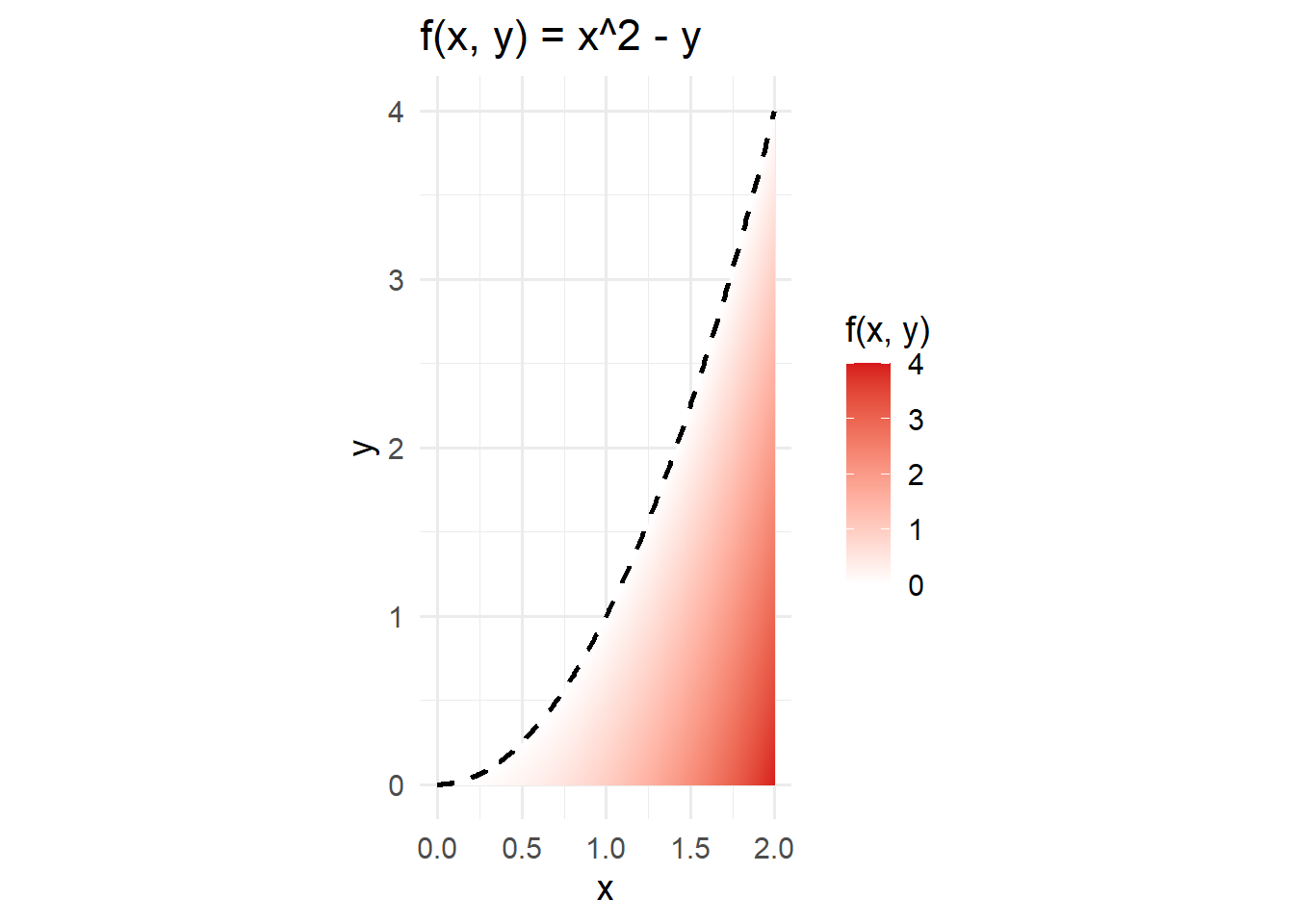
1. Write the double integral that represents the net accumulation of \(f(x,y)\) over the region.
   
2. Evaluate the integral.
   
3. Determine whether the function changes sign inside the region.
   
4. Now compute the total geometric magnitude \(\displaystyle \iint_R |x^2 - y|\, dA\).
   
5. Explain why the two answers differ (if they do).
   

---

Problem 4 — Triple Integral with Nonlinear Density

A solid occupies the region \[ 0 \le x \le 1,\quad 0 \le y \le x,\quad 0 \le z \le x+y. \]

Density varies according to \[ \rho(x,y,z) = 3x^2 + yz. \]

1. Write the triple integral for the total mass of the solid.
   
2. Evaluate the integral.
   
3. Which variable would you integrate with respect to first to simplify computation?
   
4. Interpret what the inner integral represents physically.
   

---

Problem 5 — Atmospheric Mixing in a Valley (Environmental Triple Integral)

A valley is approximated by a rectangular box (units in km): \[ 0 \le x \le 4,\quad -2 \le y \le 2,\quad 0 \le z \le 1. \]

A pollutant’s concentration (mass per km\(^3\)) varies with position as \[ C(x,y,z) = e^{-z}\,(2 + x)\,|y|. \]

1. Write a triple integral that represents the total pollutant mass in the valley.
   
2. Evaluate the integral.
   
3. Explain how symmetry in \(y\) helps you simplify the computation.
   
4. In one sentence, interpret what the factor \(e^{-z}\) suggests physically.
   

---

14.16 Core Ideas Across These Problems

• Curved boundaries require careful bounds.
  
• Order of integration matters computationally.
  
• Sign changes inside a region affect net accumulation.
  
• Symmetry arguments can replace heavy computation.
  
• Absolute value removes cancellation and changes interpretation.

Click to Unlock Solutions