Chapter 16 Differential Equations
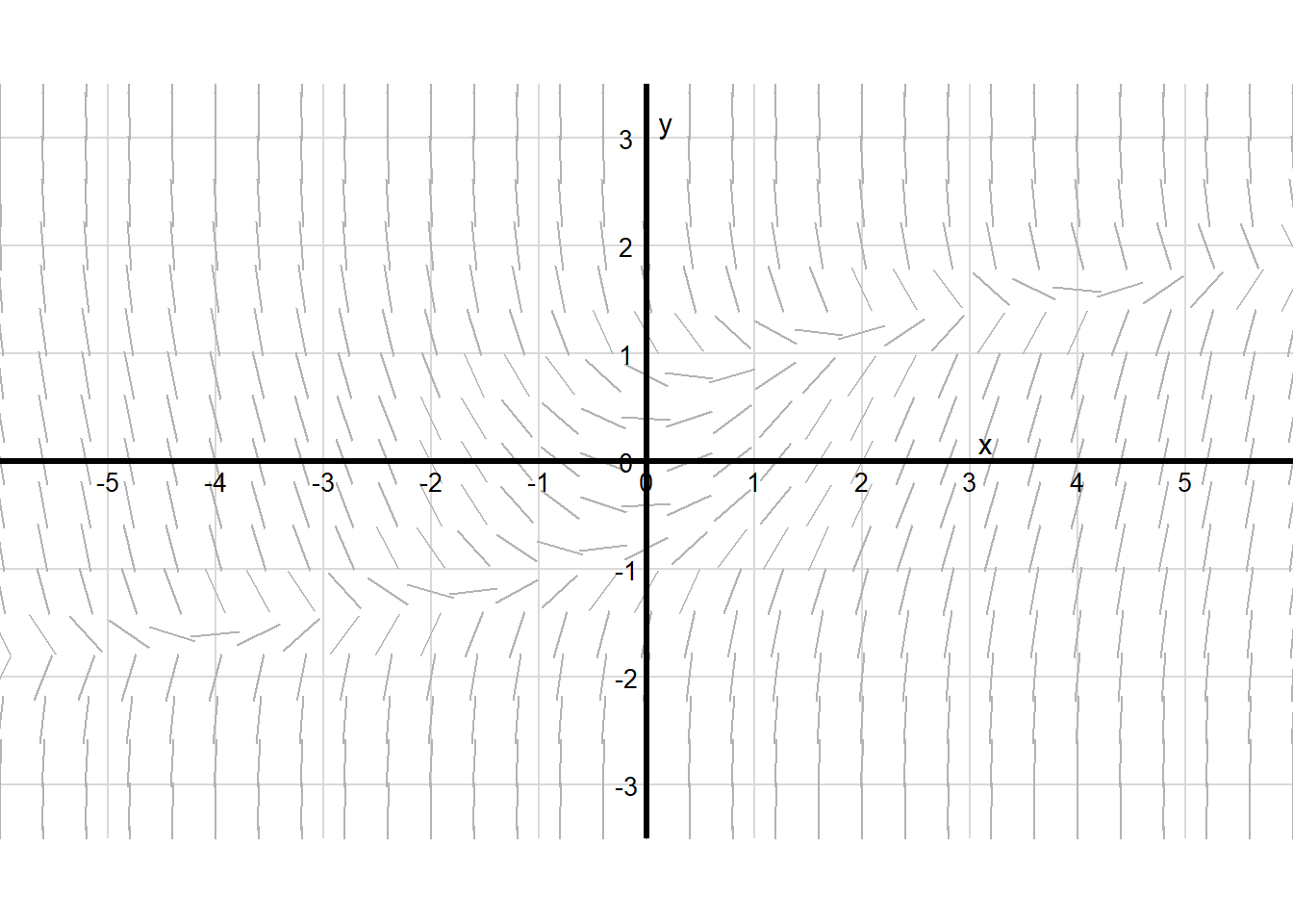
Graph 1
For each of these sketches imagine you are floating on a paddleboard.
- Make an ‘x’ anywhere on the graph
Now imagine the grey lines are the current below you
- Sketch the path you would take
- Go forwards until you leave the bounds of the graph
- Go backwards until you leave the bounds of the graph
You should now have a single trajectory.
Now repeat this process 2 more times, each time putting your ‘x’ at a different starting point.
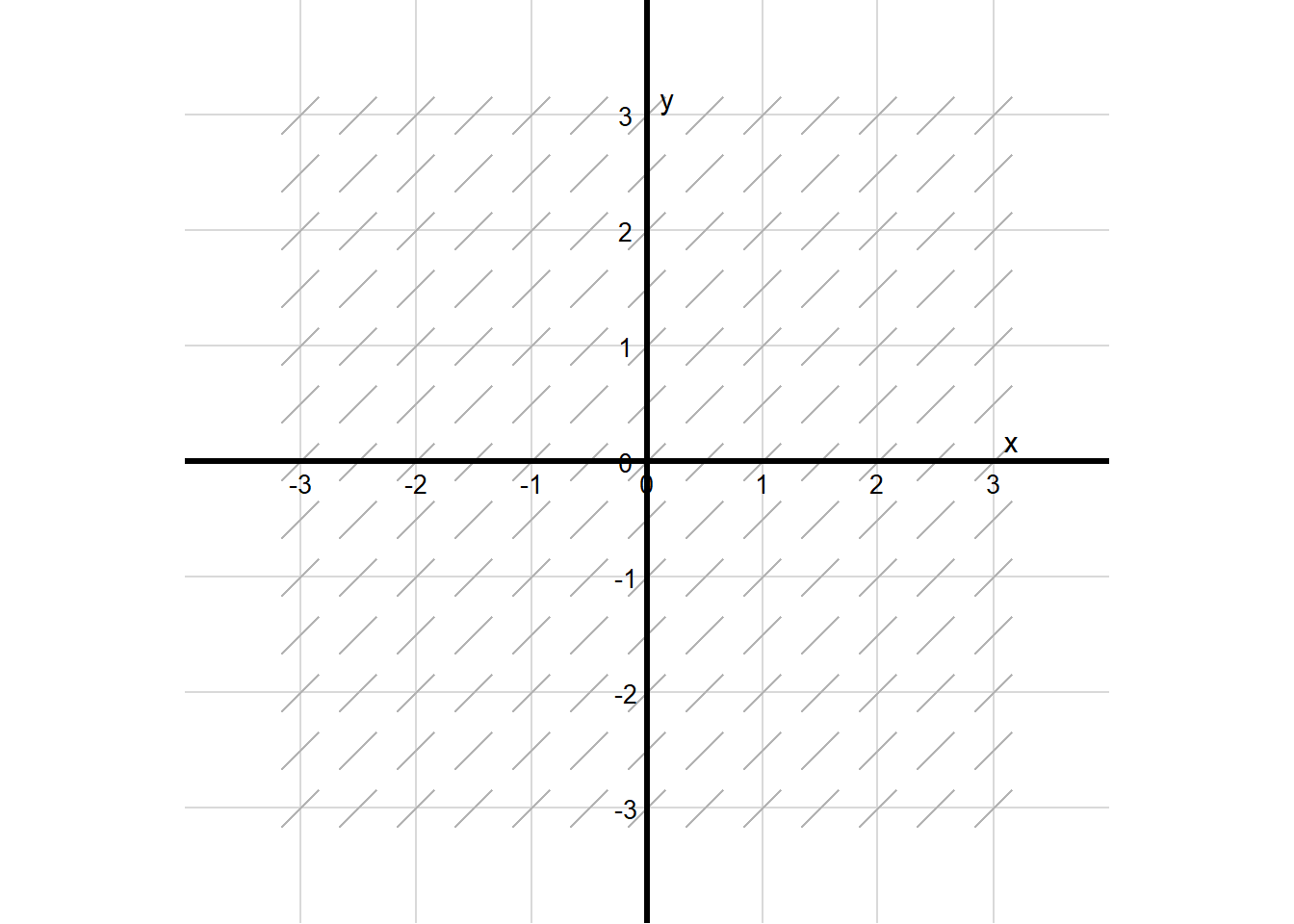
- What happens to your trajectories?
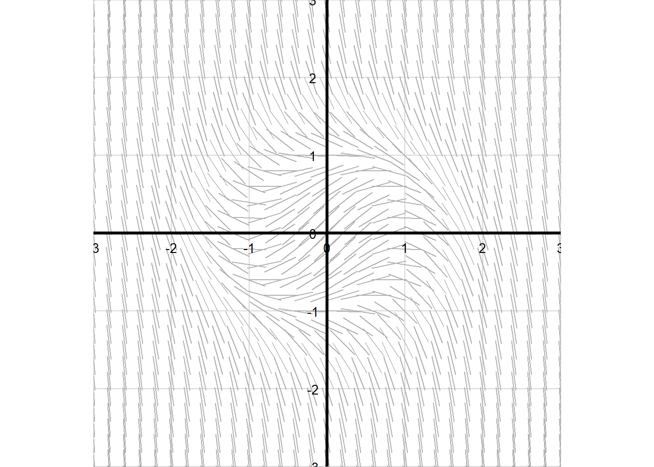
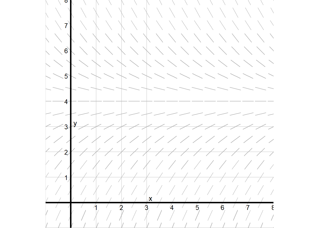
Graph 2
For this graph place 4 x’s on the left edge of the page. Sketch the trajectories you create as you move to the right.
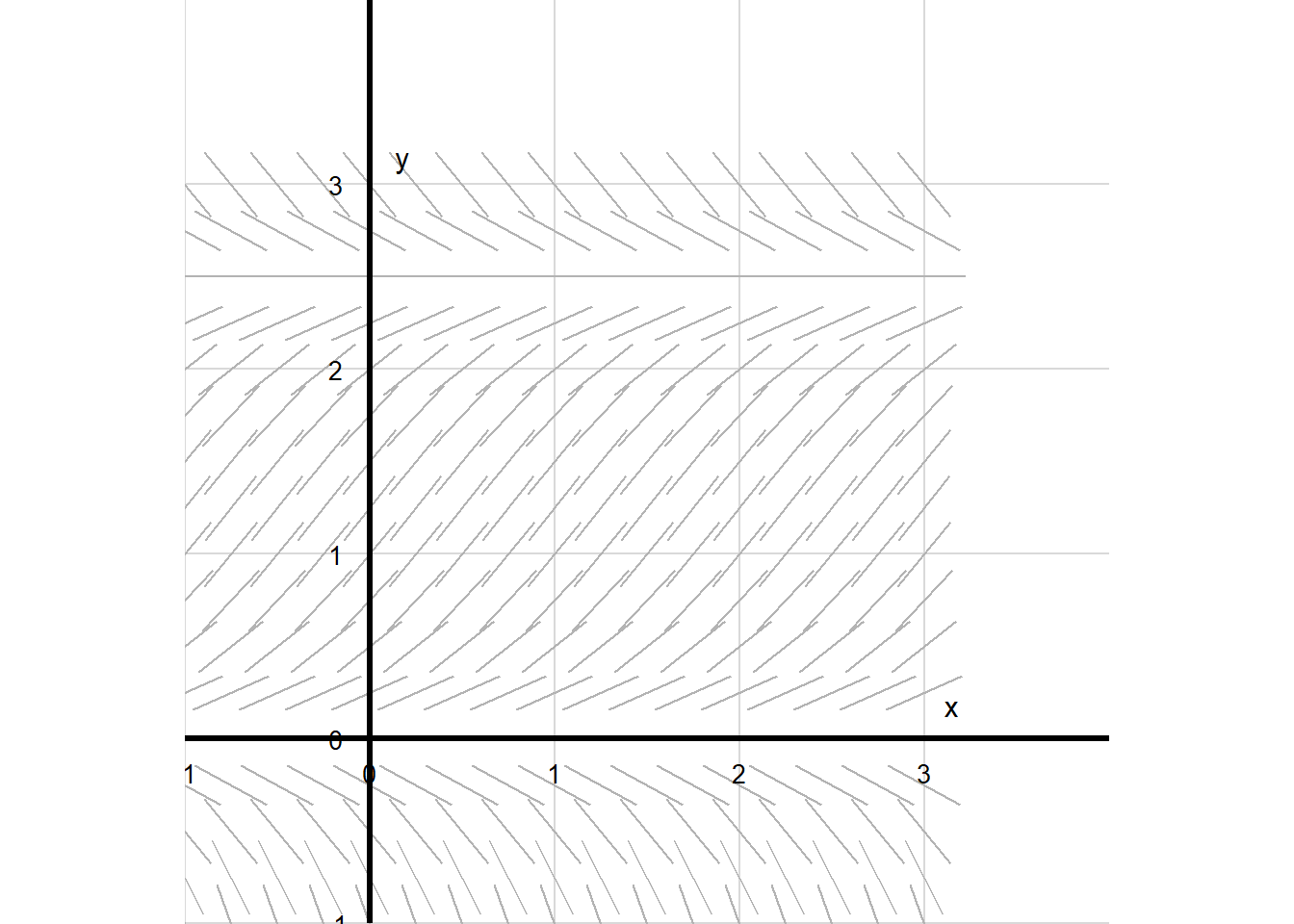
What happens if you start below the x axis?
What happens if you start between y=0 and y=2.5?
What happens if you state above y=2.5?
How would describe the y=0 line?
What about the y= 2.5 line?
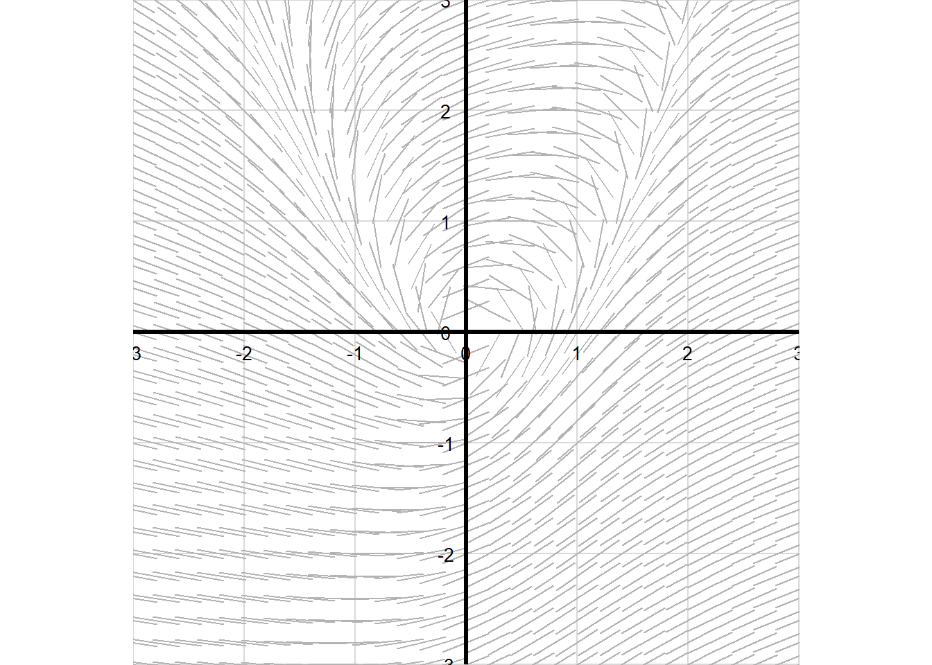
Graph 3
For this graph place 4 x’s on the left edge of the page. Sketch the trajectories you create as you move to the right.
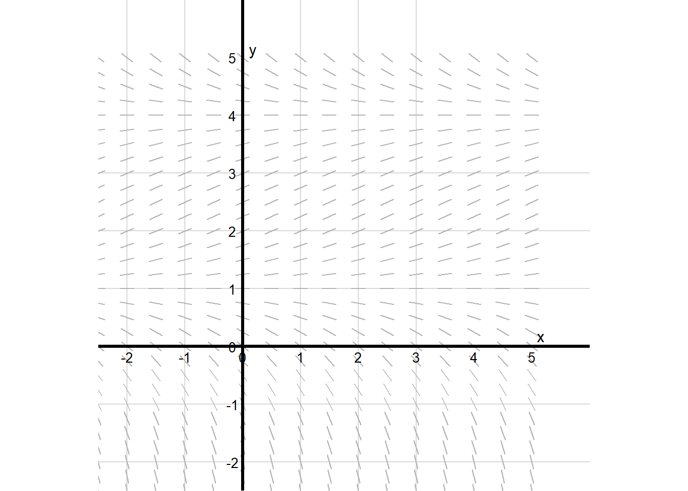
- There was a slight change between Graph 2 and Graph 3. Can you describe what happened?
Graph 4
For this graph place 4 x’s on the left edge of the page. Sketch the trajectories you create as you move to the right.
- what happens to all the trajectories by the time to get to the right?
- try and plot a line through the field were the grey lines have slope of zero (you may need to interpolate a little)
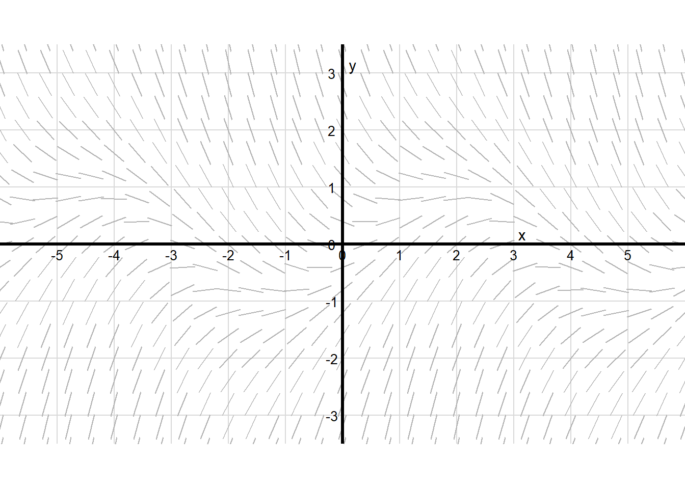
Graph 5
For this graph place 4 x’s on the left edge of the page. Sketch the trajectories you create as you move to the right.
- what happens to all the trajectories by the time to get to the right?
- try and plot a line through the field were the grey lines have slope of zero (you may need to interpolate a little)
Graph 6
For this graph place 4 x’s on the top edge of the page. Sketch the trajectories you create as you move to the right.
- what happens to all the trajectories as you move in this field?
- try and plot a line through the field were the grey lines have slope of zero (you may need to interpolate a little)
Graph 7
For this graph place 4 x’s on the top edge of the page and 4 x’s on the left edge. Sketch the trajectories you create as you move to the right.
- what happens to all the trajectories by the time to get to the right?
- try and plot a line through the field were the grey lines have slope of zero (you may need to interpolate a little)
- how would you describe (0,0)?
SUMMARY
- What do the grey lines represent?
- What does one of the trajectories represent?
- Why does trajectory vary?
- What do the different x’s represent?
- What are zero slope grey lines present?
- What does convergence indicate?
- What does divergence indicate?
16.1 Building our own slope field
Example 2
The slope field is a way to represent how a point is changing instantaneously. We can create a ‘field’ by calculating the value of the derivative on a grid.
Let’s consider \[ f'(x) = 2 \]
If I know the derivative of the function is 2 everywhere I can create a slope field

If we take the integration of f’(x)
\[ \int f'(x) dx \]
\[ \int 2 dx = 2x+c \]
So we have a family of functions that solve the differential equation.
Now this differential equation wasn’t that interesting as it was just a constant
Example 2
Now let’s consider \[ f'(x) = x \]
If I know the derivative of the function is x everywhere I can create a slope field

If we take the integration of f’(x)
\[ \int f'(x) dx \]
\[ \int x dx = \frac{x^2}{2}+c \]
So we have a family of functions that solve the differential equation.
You know how to take that antiderivative without too much trouble. Another way to do it is by using Separation of Variables. \[ \frac{dy}{dx}=x \] Now separate the variables by grouping all terms with x’s on one side and y’s on the other. Keep the dx and dy in the numerators.
\[ dy=x . dx \]
Now we are saying a small amount of y dy is equal to x times a small about of x dx. So lets accumulate these small amounts by taking the integration of both sides.
\[ \int dy= \int x . dx \]
\[ y= \frac{x^2}{2} +c \]
We get the same solution but using a slightly different methodology - this methodology know as the Separation of Variables becomes very useful when differential equations are functions of themselves.
Now this differential equation is a little more interesting but is still only a function of x.
Example 3
Now let’s consider introducing y into our derivative. What does this mean - it means our derivative is a function of both x and y \[ f'(x,y) = y \]
If I know the derivative of the function is y everywhere I can create a slope field

If we take the integration of f’(x,y)
\[ \int f'(x,y) dx \]
This is a case where separation of variables will be needed.
\[ \frac{dy}{dx}=y \]


16.2 Differential Equations — Modeling Change
- How fast is a population growing right now?
- How much carbon accumulated over a decade?
- How does a system evolve over time if we only know how it changes?
Think-Pair-Share
- Which of these is a derivative question?
- Which is an integral question?
- What would the third one require?
16.3 From Rate to Rule
Consider:
\[ \frac{dy}{dt} = 4 \]
Questions
- If the rate is always 4, what must the function look like?
- What kind of graph would this produce?
Integrate:
\[ y = 4t + C \]
- Why is there a \(+C\)?
- What does \(C\) represent physically?
A differential equation gives us a rule for change.
The solution is a family of functions.
16.4 Proportional Growth
Consider:
\[ \frac{dP}{dt} = 0.4P \]
Questions Before Solving
- If \(P\) is large, what happens to the rate?
- If \(P\) is small?
- Is this constant growth or accelerating growth?
Separate variables:
\[ \frac{1}{P} dP = 0.4 dt \]
Integrate:
\[ \ln |P| = 0.4t + C \]
\[ P = Ce^{0.4t} \]
Discussion Questions
- Why is this exponential?
- What does the \(0.4\) mean in plain language?
- What are the units of \(0.4\)?
- How is \[ \frac{dP}{dt} = 0.4P \] different to \[ \frac{dP}{dt} = 0.4t \]
16.5 Proportional Decay
\[ \frac{dP}{dt} = -0.3P \]
Questions
- What changes if we flip the sign?
- What happens as \(t \to \infty\)?
Exponential growth and decay share the same structure — only the sign changes the long-term behavior.
16.6 Understanding Without Solving: Slope Fields
Consider:
\[ \frac{dP}{dt} = -0.5P + 2 \]
Evaluate the Sign of the Slope
- At \(P = 0\)
- At \(P = 4\)
- At \(P = 6\)
Create a sign table:
| \(P\) | Sign of \(dP/dt\) |
|---|---|
| 0 | |
| 4 | |
| 6 |
Discussion
- If slope is positive below 4 and negative above 4, what happens over time?
- Is \(P = 4\) stable or unstable?
16.7 Equilibrium and Stability
An equilibrium occurs when:
\[ \frac{dP}{dt} = 0 \]
Questions
- What does this mean physically?
- What does a solution look like if slope is zero everywhere?
16.8 Logistic Growth
\[ \frac{dP}{dt} = rP\left(1 - \frac{P}{K}\right) \]
Find Equilibria
- When is this equal to zero?
- How many equilibria exist?
Stability Questions
- If \(P\) is slightly above 0, what happens?
- If \(P\) is slightly above \(K\), what happens?
16.8.1 Growth as a Function of Population
Rewrite the growth term:
\[ G(P) = rP - \frac{r}{K}P^2 \]
Questions
- What type of function is this in \(P\)?
- Where does this function reach its maximum?
The maximum occurs at:
\[ P = \frac{K}{2} \]
Discussion
- Why is growth fastest at half capacity?
- Why not at maximum population?
16.9 Adding Harvesting
\[ \frac{dP}{dt} = rP\left(1 - \frac{P}{K}\right) - H \]
Questions
- What does the \(-H\) term represent?
- Is it proportional or constant?
Maximum natural growth occurs at:
\[ \frac{rK}{4} \]
Discussion
- If \(H\) is larger than this value, what must happen?
- Can the system recover?
- If \(H\) is slightly less, what changes?
- Is there a threshold population?
16.10 Structural Thinking
Discuss in pairs:
- What is the difference between solving a differential equation and analyzing its structure?
- What can slope fields tell you without solving?
- Why are nonlinear models often more realistic?
16.11 Big Picture
- Derivative → rate
- Integral → accumulation
- Differential equation → rule for change
We move from computing change to modeling entire systems.
Final Reflection
If you were modeling climate, fisheries, disease, or carbon cycles — what matters more:
- The exact formula?
- Or the structure of the system?
16.12 Modeling Heat Transfer with Differential Equations
Today we are going to build a differential equation from physical reasoning.
We will observe how hot water cools and ask:
What determines the rate at which temperature changes?
Part 1 — Brainstorming the Rate Law
Let: \[ T(t) = \text{temperature of the water} \]
We are trying to model:
\[ \frac{dT}{dt} \]
Part 2 — Three Possible Models
Based on our discussion, we will test three candidate differential equations.
Model A — Constant Cooling Rate
Assumption:
The temperature decreases at a constant rate.
\[ \frac{dT}{dt} = -c \]
Questions:
- What does this assume about the physics?
- What kind of graph does this produce?
Model B — Proportional to Temperature
Assumption:
The rate of cooling is proportional to the current temperature.
\[ \frac{dT}{dt} = -rT \]
Questions:
- What physical situation would make this reasonable?
- What does this assume about the environment?
Model C — Proportional to Temperature Difference
Assumption:
The cooling rate depends on how different the water is from the surrounding room.
Let: \[ T_s = \text{room temperature} \]
\[ \frac{dT}{dt} = -k(T - T_s) \]
Questions:
- Why subtract \(T_s\)?
- Why does this make more physical sense than Model B?
Part 3 — Compare the Assumptions
Fill in this table:
| Model | Long-Term Behavior | Physical Issue |
|---|---|---|
| A | ||
| B | ||
| C |
Discuss:
- Which model predicts temperature going below room temperature?
- Which model predicts temperature approaching zero?
- Which model predicts temperature approaching room temperature?
Part 4 — From Differential Equation to Temperature Model \(T(t)\)
We now have three proposed differential equations.
Our goal is to turn each one into a usable formula for:
\[ T(t) \]
Before we start solving, let’s be clear about the steps.
What Are We Trying to Do?
For each model, we want to:
- Solve the differential equation.
- Use any information we know at the start.
- Identify what constants remain unknown.
- Think about how we could determine those constants from data.
What Do We Already Know?
We know:
\[ T(0) = T_0 \]
So at time zero, the temperature equals the initial temperature.
This is called an initial condition.
That piece of information will allow us to determine one constant in each solution.
How Do We Solve These Equations?
All three equations are first-order differential equations.
For Models B and C, we will:
- Separate variables.
- Integrate both sides.
- Solve for \(T(t)\).
- Use the initial condition to determine the constant.
For Model A, the equation is already easy to integrate directly.
As we work, ask yourself:
- What constant appears after integrating?
- What does it represent physically?
- What information do we still need to determine it?
Model A: Constant Cooling Rate
Differential equation:
\[ \frac{dT}{dt} = -c \]
What Is Still Unknown?
The constant \(c\).
Questions:
- What does \(c\) represent physically?
- How could we determine \(c\) using measurements?
What Is Still Unknown?
The constant \(r\).
Questions:
- What does \(r\) control in this model?
- If we measure temperature after 5 minutes, could we solve for \(r\)?
- How?
Model C: Rate Proportional to Temperature Difference
Differential equation:
\[ \frac{dT}{dt} = -k(T - T_s) \]
What Is Still Unknown?
The constant \(k\).
Questions:
- What physical property might affect \(k\)?
- How could we use our 5-minute measurement to determine \(k\)?
- Why does this model behave differently from Model B in the long term?
Big Picture
After solving each equation:
- We used the initial condition to determine one constant.
- One parameter remains unknown in each model.
- That remaining parameter must be determined from data.
So the next question becomes:
How can we use our measurements to estimate the rate constants?
That is where modeling meets experiment.
How could we find c, r and k?
DATA! If we had another measurement at known time we would have only one unknown in each of those equations.
Demo Data
From the demo
Paper Cup
- Starting Temperature =
- 1st Measurement =
- Time of Measurement =
Metal Mug
- Starting Temperature =
- 1st Measurement =
- Time of Measurement =
Polystyrene
- Starting Temperature =
- 1st Measurement =
- Time of Measurement =
Can you predict the temperature of the three cups at
t=60mins
16.13 Real-World Application: How Fast Does Permafrost Respond to Warming?
We just modeled how hot water cools toward room temperature.
Now we will apply the same mathematical structure to a real environmental system: permafrost.
Permafrost is ground that remains frozen (below 0°C) for at least two consecutive years.
As Arctic air temperatures rise, the ground begins to warm.
But does it warm instantly?
Step 1 — Define the Variables
Let:
\[ T_g(t) = \text{ground temperature (°C)} \]
\[ T_a = \text{air temperature (°C)} \]
Assume the rate at which ground temperature changes depends on how different it is from the air temperature.
Write the model:
\[ \frac{dT_g}{dt} = -k(T_g - T_a) \]
Step 2 — What Does This Model Mean?
Discuss:
- What does the parameter \(k\) represent physically?
- What would make \(k\) larger?
- What would make \(k\) smaller?
- If \(T_g = T_a\), what happens?
Step 3 — Solve the Differential Equation
We already know how to solve this type of equation.
The solution is:
\[ T_g(t) = T_a + (T_{g0} - T_a)e^{-kt} \]
Where:
- \(T_{g0}\) is the initial ground temperature.
- \(k\) controls how fast the ground adjusts.
Step 4 — Apply a Climate Change Scenario
Suppose:
Initial ground temperature: \[ T_g(0) = -4^\circ C \]
New average air temperature after warming: \[ T_a = 0^\circ C \]
Estimated thermal coupling constant: \[ k = 0.15 \text{ per year} \]
Question 1
How long until the ground warms to \(-1^\circ C\)?
Set:
\[ -1 = -4e^{-0.15t} \]
Solve for \(t\).
Steps:
\[ \frac{1}{4} = e^{-0.15t} \]
\[ \ln\left(\frac{1}{4}\right) = -0.15t \]
\[ t = \frac{\ln(4)}{0.15} \]
Compute this value.
Step 6 — Interpret the Result
- Does the ground instantly warm when air warms?
- What determines how quickly it responds?
- If \(k\) were smaller, what would happen to the response time?
- If \(k\) were larger, what would happen?
Step 7 — Thinking Bigger
Permafrost stores large amounts of carbon.
If warming causes ground temperature to approach 0°C more quickly:
- What might happen to stored carbon?
- What feedbacks might occur?
Final Reflection
We used the same differential equation structure as the hot water in a cup.
In the cup:
- The system relaxed toward room temperature.
In permafrost:
- The ground relaxes toward air temperature.
The mathematics is identical.
Only the context changed.
This is the power of differential equations: they describe structure that appears across very different systems.
Part I - Matching Slope Fields
Things to think about
- Identify where the equilibrium points are in the differential equation
- Think about symmetry; ask “does the slope change in x, in y, or in x and y”
- Calculate the derivative at a few test points
- check for sign and magnitude
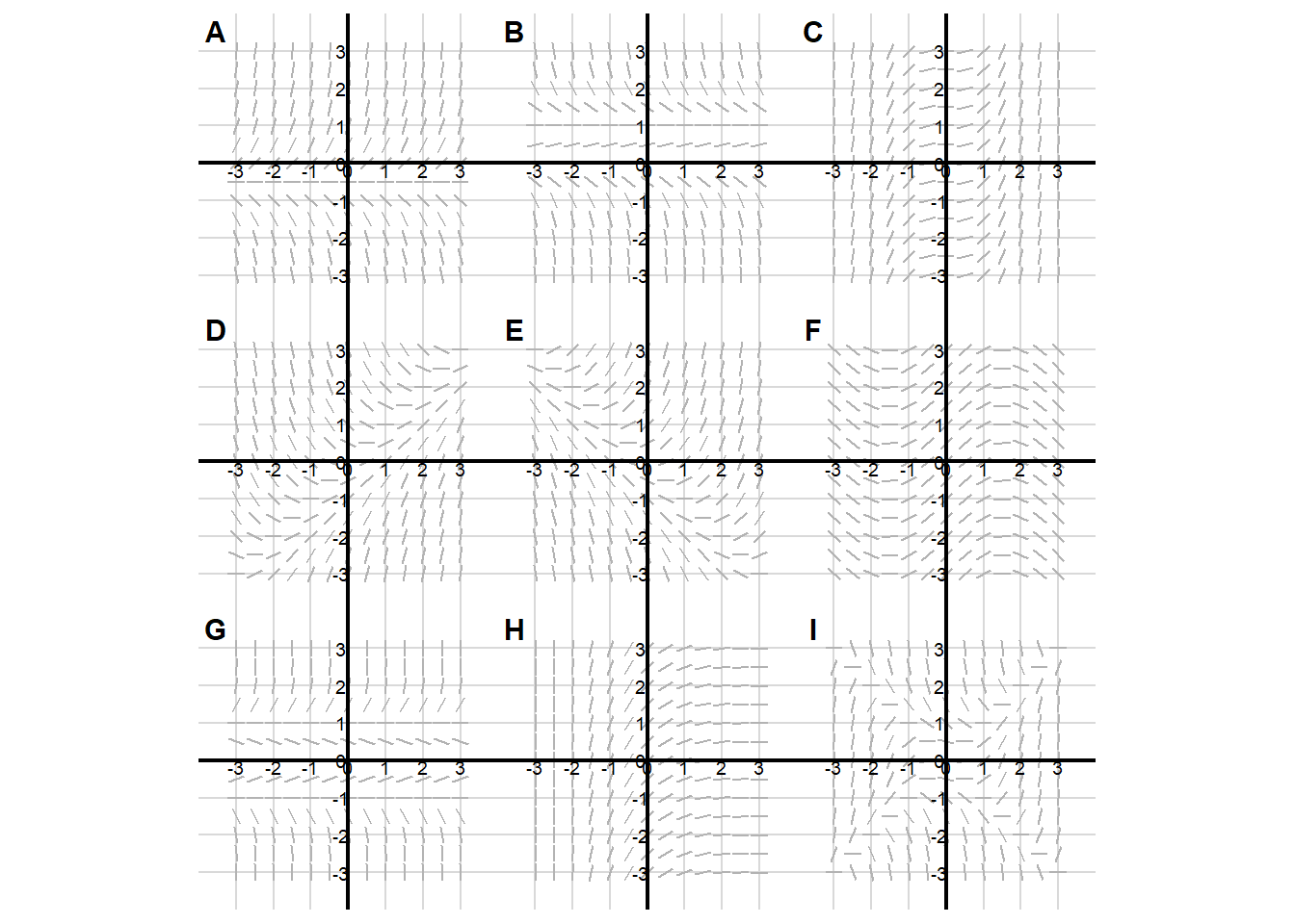
Differential Equations (Match with Slope Fields)
Write the letter of the slope field (A–I) that matches each differential equation.
| Equation | Matching Slope Field |
|---|---|
| \[\dfrac{dy}{dx} = x + y\] | |
| \[\dfrac{dy}{dx} = e^{-x}\] | |
| \[\dfrac{dy}{dx} = y(1-y)\] | |
| \[\dfrac{dy}{dx} = x^2 - y^2\] | |
| \[\dfrac{dy}{dx} = 2y + 1\] | |
| \[\dfrac{dy}{dx} = \cos(x)\] | |
| \[\dfrac{dy}{dx} = x^2\] | |
| \[\dfrac{dy}{dx} = y^3 - y\] | |
| \[\dfrac{dy}{dx} = x - y\] |
Part II. Separation of Variables Practice
Solve each differential equation using separation of variables.
Include the constant of integration. If an initial condition is given, find the specific solution.
Problems are ordered roughly from easiest to hardest.
Basic exponential growth \[ \dfrac{dy}{dt}=3y \]
Basic exponential decay \[ \dfrac{dy}{dt}=-0.6y \]
Power of \(t\) times \(y\) \[ \dfrac{dy}{dt}=t\,y \]
State dependence with a shift \[ \dfrac{dy}{dt}=2(y-1) \]
Product of \(t\) and a shifted state \[ \dfrac{dy}{dt}=t(y+2) \]
Rational state dependence \[ \dfrac{dy}{dt}=\frac{y}{1+y} \]
Quadratic nonlinearity \[ \dfrac{dy}{dt}=y^2 \]
Quadratic with a shift (requires partial fractions) \[ \dfrac{dy}{dt}=y^2-1 \]
Logistic-style structure (partial fractions) \[ \dfrac{dP}{dt}=P(4-P) \]
Mixed time and logistic-style state dependence \[ \dfrac{dP}{dt}=t\,P(3-P) \]
11
When solving a differential equation using separation of variables, what is the main goal of the separation step?
Rewrite the equation so that all \(y\) terms are with \(dy\) and all \(t\) terms are with \(dt\)
Eliminate the derivative from the equation
Move all constants to the left side of the equation
Make the equation linear
12
Consider
\[ \dfrac{dy}{dt} = ty \]
What is the correct first step in separating variables?
\(y\,dy = t\,dt\)
\(\dfrac{1}{y}dy = t\,dt\)
\(dy = ty\,dt\)
\(\dfrac{1}{t}dy = y\,dt\)
13
After separating variables, why are we allowed to integrate both sides of the equation?
Because the derivative has been eliminated
Because both sides now represent differentials of the same variable
Because each side now depends on only one variable, so each can be integrated independently
Because the equation becomes algebraic
14
When solving
\[ \dfrac{dy}{dt} = 2y \]
the step
\[ \frac{1}{y}dy = 2dt \]
is useful because it allows us to integrate
\(y\) with respect to \(t\)
\(y\) with respect to \(y\)
each variable with respect to its own differential
both sides with respect to \(t\)
15
After integrating both sides of a separated equation we obtain
\[ \ln|y| = 3t + C \]
Why do we usually rewrite the solution as
\[ y = Ce^{3t} \]
Because exponential form is easier to differentiate
Because solving for \(y\) gives a clearer expression for the function
Because logarithms cannot contain constants
Because separation of variables requires exponential solutions
Part III. Separation of Variables with Initial Conditions
Solve each differential equation using separation of variables.
Then use the initial condition to determine the constant and write the specific solution.
- \[ \frac{dy}{dt} = 2y, \qquad y(0)=5 \]
- \[ \frac{dy}{dt} = -0.5y, \qquad y(0)=12 \]
- \[ \frac{dy}{dt} = t\,y, \qquad y(0)=4 \]
- \[ \frac{dy}{dt} = 3(y-2), \qquad y(0)=5 \]
- \[ \frac{dy}{dt} = t(y+1), \qquad y(0)=0 \]
- \[ \frac{dy}{dt} = y^2, \qquad y(0)=2 \]
- \[ \frac{dy}{dt} = y^2-4, \qquad y(0)=3 \]
- \[ \frac{dP}{dt} = P(5-P), \qquad P(0)=1 \]
- \[ \frac{dP}{dt} = P(3-P), \qquad P(0)=2 \]
- \[ \frac{dP}{dt} = t\,P(4-P), \qquad P(0)=1 \]
11. What is the purpose of the initial condition in an initial value problem (IVP)?
It helps separate the variables correctly.
It determines the constant of integration so that the solution matches the starting value.
It changes the differential equation itself.
It makes the solution easier to integrate.
12. Why do we separate variables before integrating in these problems?
It guarantees the solution will be linear.
It allows us to integrate each variable independently on different sides of the equation.
It removes the constant of integration.
It ensures the solution will be exponential.
13. When solving
\[ \frac{dy}{dt} = ky \]
why does the solution always take the form \(y = Ce^{kt}\)?
Because the derivative of \(e^{kt}\) is proportional to itself.
Because exponentials are the only functions we know how to integrate.
Because the constant \(k\) forces the solution to be exponential.
Because all differential equations produce exponential solutions.
14. When solving a differential equation using separation of variables, where does the constant of integration come from?
From the original differential equation.
From the initial condition.
From the integration step.
From rewriting the equation in separated form.
15. Why do we substitute the initial condition after integrating rather than before?
Because the equation cannot be separated until after integration.
Because the constant of integration does not appear until after we integrate.
Because the initial condition changes the derivative.
Because the integration rules require a value for the constant first.
16. When separating variables and integrating both sides, it looks like we should get two constants of integration. Why do we usually write only one constant in the final solution?
Because the two constants cancel each other out.
Because constants from both sides can be combined into a single new constant.
Because one constant always equals zero.
Because the initial condition removes one of the constants automatically.
Part IV. Determining the Rate Constant from Two Points
For each problem below:
- Solve the differential equation.
- Use the initial condition to determine the constant of integration.
- Use the second data point to determine the rate constant.
Write the final function describing the system.
\[ \frac{dy}{dt} = ky \]
\[ y(0) = 4, \qquad y(3) = 20 \]
\[ \frac{dP}{dt} = kP \]
\[ P(0) = 10, \qquad P(5) = 80 \]
\[ \frac{dN}{dt} = kN \]
\[ N(0) = 6, \qquad N(4) = 18 \]
\[ \frac{dC}{dt} = kC \]
\[ C(0) = 12, \qquad C(2) = 9 \]
\[ \frac{dP}{dt} = kP \]
\[ P(0) = 5, \qquad P(6) = 15 \]
After solving
\[ \frac{dy}{dt}=ky \]
we obtain
\[ y = Ce^{kt} \]
Which piece of information determines the constant \(C\)?
The differential equation
The initial condition
The second data point
The value of \(k\)
Once the constant \(C\) is known, what is the purpose of the second data point?
It determines the rate constant \(k\)
It confirms that the derivative is correct
It changes the constant \(C\)
It determines the time variable
After solving a differential equation and applying the initial condition, we obtain a model like
\[ y = 8e^{kt} \]
Why do we still need another data point?
To verify the solution method
To determine the value of the rate constant \(k\)
To calculate the derivative
To eliminate the exponential function
Part V. Slope Fields, Equilibria, and Stability
(No explicit solving required. Use sign reasoning and interpretation.)
In this section, you are not asked to solve the differential equations algebraically. Instead, focus on understanding how the rate of change depends on the current value of the variable, and use that to predict behavior.
1) Interpreting the sign of the rate
Consider the differential equation:
\[ \dfrac{dN}{dt} = -0.3N + 9. \]
For each value of \(N\), determine whether the solution is increasing, decreasing, or momentarily constant. Explain your reasoning using the sign of the derivative.
- \(N = 0\)
- \(N = 10\)
- \(N = 30\)
- \(N = 40\)
2) Equilibrium and long-term behavior
Using
\[ \dfrac{dN}{dt} = -0.3N + 9, \]
- Find the equilibrium value \(N^*\).
- Classify it as stable or unstable using sign reasoning.
- Sketch a one-dimensional direction diagram (arrows on the \(N\)-axis).
- Predict the long-term behavior for different initial values of \(N\).
3) Logistic-style equilibrium reasoning
Consider the differential equation:
\[ \dfrac{dP}{dt} = P(6 - P). \]
- Find all equilibrium values.
- Use sign reasoning to determine whether each equilibrium is stable or unstable.
- Draw a direction diagram on the \(P\)-axis.
- Describe what happens to the population if:
- \(P(0)=2\)
- \(P(0)=5\)
- \(P(0)=8\)
4) Multiple equilibria and thresholds
Consider
\[ \dfrac{dP}{dt} = P(4 - P)(P - 1). \]
- Find all equilibrium values.
- Determine the sign of \(dP/dt\) in each interval between equilibria.
- Classify each equilibrium as stable or unstable.
- Predict the long-term behavior if:
- \(P(0)=0.5\)
- \(P(0)=2\)
- \(P(0)=5\)
Explain your reasoning using sign patterns and direction arrows.
Solution Key
Answer Key
Part II (Separation of Variables)
- \(\dfrac{dy}{dt}=3y\)
Separate and integrate: \[ \frac{1}{y}\,dy = 3\,dt \] \[ \ln|y| = 3t + C \] Exponentiate: \[ y = Ce^{3t} \]
- \(\dfrac{dy}{dt}=-0.6y\)
\[ \frac{1}{y}\,dy = -0.6\,dt \] \[ \ln|y| = -0.6t + C \] \[ y = Ce^{-0.6t} \]
- \(\dfrac{dy}{dt}=t\,y\)
\[ \frac{1}{y}\,dy = t\,dt \] \[ \ln|y| = \frac{t^2}{2} + C \] \[ y = Ce^{t^2/2} \]
- \(\dfrac{dy}{dt}=2(y-1)\)
\[ \frac{1}{y-1}\,dy = 2\,dt \] \[ \ln|y-1| = 2t + C \] \[ y - 1 = Ce^{2t} \] \[ y = 1 + Ce^{2t} \]
- \(\dfrac{dy}{dt}=t(y+2)\)
\[ \frac{1}{y+2}\,dy = t\,dt \] \[ \ln|y+2| = \frac{t^2}{2} + C \] \[ y+2 = Ce^{t^2/2} \] \[ y = -2 + Ce^{t^2/2} \]
- \(\dfrac{dy}{dt}=\dfrac{y}{1+y}\)
Separate: \[ \frac{1+y}{y}\,dy = dt \] Rewrite: \[ \left(\frac{1}{y}+1\right)dy = dt \] Integrate: \[ \ln|y| + y = t + C \]
So the (implicit) solution is: \[ \boxed{\ln|y| + y = t + C} \] (An explicit formula for \(y(t)\) is not elementary.)
- \(\dfrac{dy}{dt}=y^2\)
\[ \frac{1}{y^2}\,dy = dt \] \[ \int y^{-2}\,dy = \int 1\,dt \] \[ -\,\frac{1}{y} = t + C \] Solve for \(y\): \[ \frac{1}{y} = -t + C \] \[ y = \frac{1}{C - t} \]
- \(\dfrac{dy}{dt}=y^2-1\)
Separate: \[ \frac{dy}{y^2-1}=dt \] Use partial fractions: \[ \frac{1}{y^2-1}=\frac{1}{(y-1)(y+1)} =\frac{1}{2}\left(\frac{1}{y-1}-\frac{1}{y+1}\right) \] Integrate: \[ \int \frac{dy}{y^2-1} = \frac{1}{2}\int\left(\frac{1}{y-1}-\frac{1}{y+1}\right)dy = t + C \] \[ \frac{1}{2}\left(\ln|y-1|-\ln|y+1|\right)=t+C \] \[ \frac{1}{2}\ln\left|\frac{y-1}{y+1}\right|=t+C \] \[ \ln\left|\frac{y-1}{y+1}\right|=2t+C \] Equivalent implicit form: \[ \boxed{\frac{y-1}{y+1}=Ce^{2t}} \]
- \(\dfrac{dP}{dt}=P(4-P)\)
Separate: \[ \frac{dP}{P(4-P)}=dt \] Partial fractions: \[ \frac{1}{P(4-P)}=\frac{1}{4}\left(\frac{1}{P}+\frac{1}{4-P}\right) \] Integrate: \[ \int \frac{dP}{P(4-P)} =\frac{1}{4}\int\left(\frac{1}{P}+\frac{1}{4-P}\right)dP = t + C \] \[ \frac{1}{4}\left(\ln|P|-\ln|4-P|\right)=t+C \] \[ \frac{1}{4}\ln\left|\frac{P}{4-P}\right|=t+C \] \[ \ln\left|\frac{P}{4-P}\right|=4t+C \] Equivalent implicit form: \[ \boxed{\frac{P}{4-P}=Ce^{4t}} \] (You can solve explicitly if desired.)
- \(\dfrac{dP}{dt}=t\,P(3-P)\)
Separate: \[ \frac{dP}{P(3-P)} = t\,dt \] Partial fractions: \[ \frac{1}{P(3-P)}=\frac{1}{3}\left(\frac{1}{P}+\frac{1}{3-P}\right) \] Integrate both sides: \[ \frac{1}{3}\int\left(\frac{1}{P}+\frac{1}{3-P}\right)dP = \int t\,dt \] \[ \frac{1}{3}\left(\ln|P|-\ln|3-P|\right)=\frac{t^2}{2}+C \] \[ \frac{1}{3}\ln\left|\frac{P}{3-P}\right|=\frac{t^2}{2}+C \] \[ \ln\left|\frac{P}{3-P}\right|=\frac{3}{2}t^2 + C \] Equivalent implicit form: \[ \boxed{\frac{P}{3-P}=Ce^{\frac{3}{2}t^2}} \]
- A
- B
- C
- C
- B
Part III (Separation of Variables with IVPs)
- \[ \frac{dy}{dt}=2y, \quad y(0)=5 \]
Separate: \[ \frac{1}{y}dy = 2dt \]
Integrate: \[ \ln|y| = 2t + C \]
Exponentiate: \[ y = Ce^{2t} \]
Apply initial condition:
\[ 5 = Ce^0 \]
\[ C = 5 \]
Final solution:
\[ y = 5e^{2t} \]
- \[ \frac{dy}{dt}=-0.5y, \quad y(0)=12 \]
Separate: \[ \frac{1}{y}dy = -0.5dt \]
Integrate: \[ \ln|y| = -0.5t + C \]
\[ y = Ce^{-0.5t} \]
Initial condition:
\[ 12 = C \]
Solution:
\[ y = 12e^{-0.5t} \]
- \[ \frac{dy}{dt}=ty, \quad y(0)=4 \]
Separate:
\[ \frac{1}{y}dy = tdt \]
Integrate:
\[ \ln|y| = \frac{t^2}{2} + C \]
\[ y = Ce^{t^2/2} \]
Initial condition:
\[ 4 = C \]
Solution:
\[ y = 4e^{t^2/2} \]
- \[ \frac{dy}{dt}=3(y-2), \quad y(0)=5 \]
Separate:
\[ \frac{1}{y-2}dy = 3dt \]
Integrate:
\[ \ln|y-2| = 3t + C \]
\[ y-2 = Ce^{3t} \]
Initial condition:
\[ 3 = C \]
Solution:
\[ y = 2 + 3e^{3t} \]
\[ \frac{dy}{dt}=t(y+1), \quad y(0)=0 \]
Separate:
\[ \frac{1}{y+1}dy = tdt \]
Integrate:
\[ \ln|y+1| = \frac{t^2}{2} + C \]
\[ y+1 = Ce^{t^2/2} \]
Initial condition:
\[ 1 = C \]
Solution:
\[ y = e^{t^2/2} - 1 \]
\[ \frac{dy}{dt}=y^2, \quad y(0)=2 \]
Separate:
\[ \frac{1}{y^2}dy = dt \]
Integrate:
\[ -\frac{1}{y} = t + C \]
\[ \frac{1}{y} = C - t \]
Initial condition:
\[ \frac{1}{2} = C \]
Solution:
\[ y = \frac{1}{\frac{1}{2} - t} \]
\[ \frac{dy}{dt}=y^2-4, \quad y(0)=3 \]
Separate:
\[ \frac{dy}{y^2-4} = dt \]
Factor:
\[ y^2-4=(y-2)(y+2) \]
Partial fractions:
\[ \frac{1}{y^2-4} = \frac{1}{4}\left(\frac{1}{y-2}-\frac{1}{y+2}\right) \]
Integrate:
\[ \frac{1}{4}\ln\left|\frac{y-2}{y+2}\right| = t + C \]
Initial condition:
\[ \frac{1}{4}\ln\left(\frac{1}{5}\right)=C \]
Solution (implicit):
\[ \ln\left|\frac{y-2}{y+2}\right| = 4t + \ln\left(\frac{1}{5}\right) \]
\[ \frac{dP}{dt}=P(5-P), \quad P(0)=1 \]
Separate:
\[ \frac{dP}{P(5-P)}=dt \]
Partial fractions:
\[ \frac{1}{P(5-P)}=\frac{1}{5}\left(\frac{1}{P}+\frac{1}{5-P}\right) \]
Integrate:
\[ \frac{1}{5}\ln\left|\frac{P}{5-P}\right| = t + C \]
Initial condition:
\[ \frac{1}{5}\ln\left(\frac{1}{4}\right)=C \]
Solution (implicit):
\[ \ln\left|\frac{P}{5-P}\right| = 5t + \ln\left(\frac{1}{4}\right) \]
\[ \frac{dP}{dt}=P(3-P), \quad P(0)=2 \]
Separate:
\[ \frac{dP}{P(3-P)} = dt \]
Partial fractions:
\[ \frac{1}{3}\left(\frac{1}{P}+\frac{1}{3-P}\right) \]
Integrate:
\[ \frac{1}{3}\ln\left|\frac{P}{3-P}\right| = t + C \]
Initial condition:
\[ \frac{1}{3}\ln(2)=C \]
Solution (implicit):
\[ \ln\left|\frac{P}{3-P}\right| = 3t + \ln(2) \]
\[ \frac{dP}{dt}=tP(4-P), \quad P(0)=1 \]
Separate:
\[ \frac{dP}{P(4-P)} = tdt \]
Partial fractions:
\[ \frac{1}{4}\left(\frac{1}{P}+\frac{1}{4-P}\right) \]
Integrate:
\[ \frac{1}{4}\ln\left|\frac{P}{4-P}\right| = \frac{t^2}{2} + C \]
Initial condition:
\[ \frac{1}{4}\ln\left(\frac{1}{3}\right)=C \]
Solution:
\[ \ln\left|\frac{P}{4-P}\right| = 2t^2 + \ln\left(\frac{1}{3}\right) \]
11
Answer: B
The initial condition determines the constant of integration so the solution matches the starting value.
12
Answer: B
Separating variables allows us to integrate each variable independently on opposite sides of the equation.
13
Answer: A
The exponential function is unique because its derivative is proportional to itself.
14
Answer: C
The constant appears because indefinite integrals represent a family of antiderivatives.
15
Answer: B
The constant of integration only appears after integrating, so the initial condition must be applied afterward.
16
Answer: B
When integrating both sides we technically get two constants, but they can be combined into a single new constant.
Part IV
1
\[ \frac{dy}{dt}=ky,\qquad y(0)=4,\qquad y(3)=20 \]
General solution:
\[ y = Ce^{kt} \]
Initial condition:
\[ 4 = Ce^0 \]
\[ C=4 \]
Model:
\[ y = 4e^{kt} \]
Use second point:
\[ 20 = 4e^{3k} \]
\[ 5 = e^{3k} \]
\[ k = \frac{\ln 5}{3} \]
Final model:
\[ y = 4e^{(\ln 5 /3)t} \]
2
\[ \frac{dP}{dt}=kP,\qquad P(0)=10,\qquad P(5)=80 \]
General solution:
\[ P = Ce^{kt} \]
Initial condition:
\[ 10 = C \]
\[ P = 10e^{kt} \]
Second point:
\[ 80 = 10e^{5k} \]
\[ 8 = e^{5k} \]
\[ k = \frac{\ln 8}{5} \]
Final model:
\[ P = 10e^{(\ln 8/5)t} \]
3
\[ \frac{dN}{dt}=kN,\qquad N(0)=6,\qquad N(4)=18 \]
General solution:
\[ N = Ce^{kt} \]
Initial condition:
\[ C=6 \]
\[ N = 6e^{kt} \]
Second point:
\[ 18 = 6e^{4k} \]
\[ 3 = e^{4k} \]
\[ k = \frac{\ln 3}{4} \]
Final model:
\[ N = 6e^{(\ln 3/4)t} \]
4
\[ \frac{dC}{dt}=kC,\qquad C(0)=12,\qquad C(2)=9 \]
General solution:
\[ C = Ce^{kt} \]
Initial condition:
\[ C=12 \]
\[ C(t) = 12e^{kt} \]
Second point:
\[ 9 = 12e^{2k} \]
\[ \frac{3}{4} = e^{2k} \]
\[ k = \frac{\ln(3/4)}{2} \]
Final model:
\[ C(t) = 12e^{(\ln(3/4)/2)t} \]
5
\[ \frac{dP}{dt}=kP,\qquad P(0)=5,\qquad P(6)=15 \]
General solution:
\[ P = Ce^{kt} \]
Initial condition:
\[ C=5 \]
\[ P = 5e^{kt} \]
Second point:
\[ 15 = 5e^{6k} \]
\[ 3 = e^{6k} \]
\[ k = \frac{\ln 3}{6} \]
Final model:
\[ P = 5e^{(\ln 3/6)t} \]
B
A
B
Part V
1)
\[ \dfrac{dN}{dt} = -0.3N + 9 \]
- \(N=0\)
\[ dN/dt = 9 > 0 \]
Increasing.
- \(N=10\)
\[ dN/dt = -3 + 9 = 6 > 0 \]
Increasing.
- \(N=30\)
\[ dN/dt = -9 + 9 = 0 \]
Momentarily constant (equilibrium).
- \(N=40\)
\[ dN/dt = -12 + 9 = -3 \]
Decreasing.
2)
Set \(dN/dt = 0\)
\[ -0.3N + 9 = 0 \]
\[ N^* = 30 \]
Stability:
- If \(N < 30\): slope is positive → solutions increase.
- If \(N > 30\): slope is negative → solutions decrease.
Therefore the equilibrium is stable.
Direction diagram:
\[ \rightarrow \quad 30 \quad \leftarrow \]
Long-term behavior: all solutions move toward \(N=30\).
3)
\[ \dfrac{dP}{dt} = P(6-P) \]
Equilibria:
\[ P = 0, \quad P = 6 \]
Sign analysis:
- \(0<P<6\): positive → increasing.
- \(P>6\): negative → decreasing.
Classification:
- \(P=0\): unstable
- \(P=6\): stable
Direction diagram:
\[ 0 \rightarrow \quad \rightarrow 6 \leftarrow \]
Behavior:
- \(P(0)=2\): increases toward 6
- \(P(0)=5\): increases toward 6
- \(P(0)=8\): decreases toward 6
4)
\[ \dfrac{dP}{dt} = P(4-P)(P-1) \]
Equilibria:
\[ P=0, \quad P=1, \quad P=4 \]
Sign analysis:
| Interval | Sign |
|---|---|
| \(P<0\) | negative |
| \(0<P<1\) | positive |
| \(1<P<4\) | negative |
| \(P>4\) | positive |
Classification:
- \(P=0\): unstable
- \(P=1\): stable
- \(P=4\): unstable
Direction diagram:
\[ \leftarrow 0 \rightarrow 1 \leftarrow 4 \rightarrow \]
Behavior:
- \(P(0)=0.5\): increases toward \(P=1\)
- \(P(0)=2\): decreases toward \(P=1\)
- \(P(0)=5\): increases without bound
16.15 PolleveryWhere Questions
1) If the slope field for a differential equation looks the same along every horizontal line, what does this suggest?
- The derivative depends only on \(x\)
- The derivative depends only on \(y\)
- The derivative depends on both \(x\) and \(y\)
- The derivative is constant everywhere
2) In a slope field, an equilibrium solution occurs where:
- The slopes are largest
- The slopes are zero
- The slopes change direction rapidly
- The slopes depend only on time
3) If slopes are positive below an equilibrium and negative above it, the equilibrium is:
- Stable
- Unstable
- Neutral
- Impossible to determine
4) If slopes are negative below an equilibrium and positive above it, the equilibrium is:
- Stable
- Unstable
- Neutral
- Oscillating
5) If a slope field has vertical stripes where slopes are the same for all \(y\) values at a given \(x\), the differential equation most likely has the form:
- \(\dfrac{dy}{dt} = f(y)\)
- \(\dfrac{dy}{dt} = f(x)\)
- \(\dfrac{dy}{dt} = xy\)
- \(\dfrac{dy}{dt} = y^2\)
6) The goal of separating variables is to:
- Remove constants from the equation
- Place all \(y\) terms with \(dy\) and all \(t\) terms with \(dt\)
- Eliminate derivatives
- Convert the equation to a polynomial
7) For \(\dfrac{dy}{dt} = ty\), which step correctly separates the variables?
- \(y\,dy = t\,dt\)
- \(\frac{1}{y}dy = t\,dt\)
- \(dy = ty\,dt\)
- \(\frac{1}{t}dy = y\,dt\)
8) After separating variables, why can we integrate both sides?
- The derivative disappears
- Each side now depends on only one variable
- Integration is always allowed
- The equation becomes algebraic
9) When integrating a separated equation, the constant of integration appears because:
- Integrals represent families of functions
- The derivative contains constants
- The differential equation requires it
- Exponentials introduce constants
10) After integrating \(\ln|y| = 2t + C\), why do we rewrite the solution as \(y = Ce^{2t}\)?
- It removes logarithms
- It isolates \(y\) as a function of \(t\)
- Exponentials are easier to differentiate
- The constant disappears
11) An initial condition is used to:
- Solve the differential equation
- Determine the constant of integration
- Separate the variables
- Find the derivative
12) Why is the initial condition applied after integration?
- The constant of integration does not appear until after integration
- The derivative must be removed first
- The equation must become exponential
- The variables must be separated first
13) Suppose \(y = Ce^{kt}\) and \(y(0)=5\). What is \(C\)?
- 0
- 1
- 5
- \(e^5\)
14) Why do solutions to differential equations usually contain constants?
- Because derivatives remove constants
- Because differential equations are incomplete
- Because the solution represents a family of curves
- Because exponentials require constants
15) Suppose \(y = Ce^{kt}\) and we know \(y(0)\) and \(y(t_1)\). Why do we need both values?
- One determines \(C\), the other determines \(k\)
- One verifies the derivative
- Both determine \(C\)
- Both determine \(k\)
16) If the model is \(y = 4e^{kt}\) and \(y(3)=20\), what step helps determine \(k\)?
- Substitute \(t=0\)
- Substitute \(t=3\) and solve for \(k\)
- Differentiate the equation
- Separate the variables again
17) Why does determining \(k\) usually involve taking a logarithm?
- Exponential equations must be linearized to solve for the exponent
- Logarithms remove constants
- Derivatives require logs
- Exponentials cannot be solved otherwise
18) If the solution is \(y = 10e^{0.3t}\), what does the constant 10 represent?
- The growth rate
- The initial value
- The equilibrium value
- The slope
19) If the solution is \(y = 8e^{-0.4t}\), what does the negative exponent indicate?
- Oscillation
- Growth
- Decay
- Equilibrium
20) Why are exponential functions common solutions to differential equations like \(\dfrac{dy}{dt} = ky\)?
- Exponentials are easy to integrate
- Their derivatives are proportional to themselves
- They eliminate constants
- All equations require exponentials
Answer Key
- B
- B
- A
- B
- B
- B
- B
- B
- A
- B
- B
- A
- C
- C
- A
- B
- A
- B
- C
- B