Appendix F Uncertainty Workbook
Introduction Summary: Why Models Are Always Incomplete
- A model is never “right”; it can only be useful, trustworthy enough, and honest about its uncertainty.
- No project or model is ever complete, because every model leaves things out.
- Uncertainty is not a flaw—it’s inherent in complex natural systems and present in every measurement, parameter, and equation.
- The goal is to understand where uncertainty comes from, how to represent it, and how to quantify its effects.
- Because environmental systems are variable and only partially observable, uncertainty cannot be removed—only described and communicated responsibly.
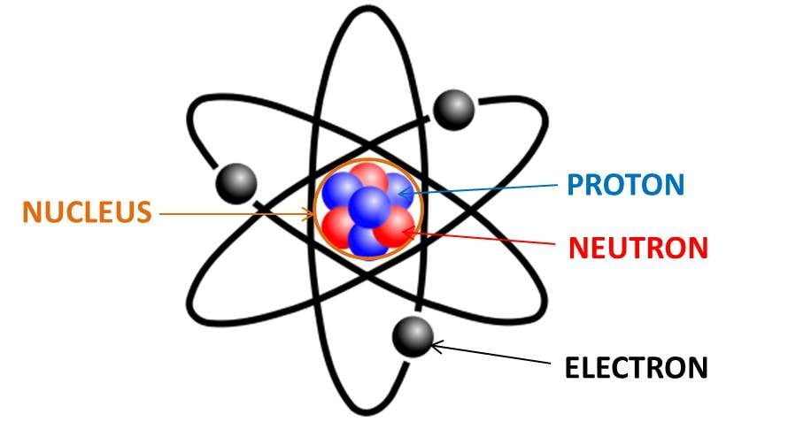
A model of an atom
Prompts for the Atom Model
- What does this atom model help you understand quickly, and why is it useful?
- What important features or behaviors of real atoms does this picture leave out?
- Why might scientists still use a simplified model even when they know it’s incomplete?
- How is this oversimplified atom model similar to the environmental models we build in this course?
Group Activity Sets: Three Environmental Models
Each group receives one model, analyzes its uncertainty, and completes a small task.
Variable definitions are included to ensure clarity without needing prior lessons.
Group 1: Soil Moisture Bucket Model
Model \[ S_{t+1} = S_t + P_t - ET_t - Q_t \]
Variable Definitions
- \(S_t\): soil moisture at time \(t\)
- \(P_t\): precipitation input
- \(ET_t\): evapotranspiration loss
- \(Q_t\): runoff
1. What’s Included?
2. What’s Left Out?
3. Where Does Uncertainty Come From?
4. List three situations** where this model would fail or mislead
Suggested Discussion Points
1. What’s Included?
- Addition of precipitation
- Loss of water through ET
- Loss of water through runoff
- A single “bucket” representing soil water storage
2. What’s Left Out?
- Soil texture and depth
- Preferential flow paths
- Root distribution and vegetation uptake specifics
- Subsurface lateral flow
- Spatial variability in precipitation
3. Where Does Uncertainty Come From?
- ET depends on many unmodeled factors
- Runoff depends on slope and saturation
- Precipitation uncertainty
- Structural simplicity (one soil layer)
4. Mini-Task
List three situations where the model would fail.
Group 2: Predator–Prey Model (Lotka–Volterra)
Model \[ \begin{aligned} \frac{dH}{dt} &= rH - aHP \\ \frac{dP}{dt} &= bHP - mP \end{aligned} \]
Variable Definitions
- \(H\): prey population (e.g., rabbits)
- \(P\): predator population (e.g., foxes)
- \(r\): prey growth rate
- \(a\): predation rate coefficient
- \(b\): predator conversion efficiency
- \(m\): predator mortality rate
1. What’s Included?
2. What’s Left Out?
3. Where Does Uncertainty Come From?
4. Mini-Task Sketch possible prey & predator curves under the same parameter set that nonetheless behave differently in the real world.
Suggested Discussion Points
1. What’s Included?
- Exponential prey growth
- Predation proportional to predator × prey encounters
- Predator growth tied to consumption of prey
- Predator mortality
- Basic feedback loop between species
2. What’s Left Out?
- Carrying capacity or resource limitation for the prey
- Seasonal changes in birth/death rates
- Age structure of either population
- Territoriality, social behavior, or hunting strategy
- Refuge areas where prey avoid predation
- Density dependence, climate effects, disease, and habitat variation
3. Where Does Uncertainty Come From?
- Prey growth rate \(r\) varies with weather, season, and food availability
- Predation rate \(a\) highly uncertain and environment-dependent
- Predator mortality \(m\) rarely constant
- Measurement error when estimating real population sizes
- Structural uncertainty: assumes perfect mixing of predators and prey
- Process uncertainty: random events like storms, disease outbreaks, or migration
4. Mini-Task
Sketch qualitative predator–prey curves under two scenarios:
1. Strong environmental variability causing prey crashes.
2. High refuge availability causing predator starvation despite abundant prey in inaccessible areas.
Explain how the simple model fails to capture these outcomes.
Group 3: Lake Temperature Energy-Balance Model
Model \[ T_{t+1} = T_t + \alpha (T_{\text{air}} - T_t) \]
Variable Definitions
- \(T_t\): lake surface temperature at time \(t\)
- \(T_{t+1}\): lake surface temperature at next time step
- \(\alpha\): heat-exchange constant
- \(T_{\text{air}}\): air temperature
1. What’s Included?
2. What’s Left Out?
3. Where Does Uncertainty Come From?
4. Identify where the model overestimates vs. underestimates warming
Suggested Discussion Points
1. What’s Included?
- Basic heat exchange
- Relaxation toward air temperature
- Single-layer assumption
2. What’s Left Out?
- Lake stratification
- Wind mixing
- Solar radiation
- Storm events
- Thermal inflows/outflows
3. Where Does Uncertainty Come From?
- Highly uncertain \(\alpha\)
- Air temperature forcing uncertainty
- Missing physical processes
- Structural simplification
4. Mini-Task
Write two conditions where warming is overestimated
and two where it is underestimated.
F.1 Why Uncertainty Matters in Modeling — Summary
- Environmental models simplify complex systems, which means something important is always left out.
- These omissions create uncertainty in model behavior and predictions.
- The goal of a model is not to perfectly mimic reality, but to provide useful, transparent guidance.
- Hiding uncertainty creates a false sense of precision and can mislead decision-making.
F.2 Summary: Major Sources of Uncertainty
- Environmental models contain multiple layers of uncertainty because they simplify complex systems and rely on imperfect information.
- Measurement uncertainty comes from errors in sensors, field instruments, and remote-sensing products; these errors affect initial conditions, calibration, and validation.
- Process uncertainty reflects the inherent randomness of nature—rainfall variability, wildfire ignition, biological growth differences—even if the model equations were perfect.
- Parameter uncertainty arises because parameters such as growth rates, reaction rates, or carrying capacities are estimated from limited or noisy data and vary over time and space.
- Structural uncertainty comes from the form of the model itself—its equations, simplifications, missing feedbacks, and unrepresented processes; it can introduce systematic error.
F.3 Summary: Additional Contributors to Uncertainty
- Initial condition uncertainty comes from not knowing the exact state of the system at the start (soil moisture, biomass, population sizes, ocean profiles).
- Small errors in starting values can grow dramatically, especially in nonlinear or chaotic systems.
- Even careful measurements (forest plots, hydrology sensors, animal surveys) can vary widely in accuracy.
- Small errors in starting values can grow dramatically, especially in nonlinear or chaotic systems.
- Forcing uncertainty arises from unknown or unpredictable inputs that drive the model (future rainfall, temperature, nutrient loads, emissions, management decisions).
- Competing forecasts or scenarios can lead to very different model outcomes, especially over long time scales.
- Numerical/computational uncertainty comes from how computers approximate equations (rounding, solver step sizes, grid resolution, Monte Carlo sampling, optimization tolerance).
- These errors are usually small but can influence results in sensitive or complex models.
- Together, these uncertainties explain why two seemingly identical models may behave differently and why precise outputs can hide deeper instability or variability.
F.4 Summary: Representing Uncertainty in Models
- Once uncertainty is identified, it must be represented explicitly in the model so predictions show a range of plausible outcomes rather than a single path.
- Stochastic models add randomness directly into the system equations, capturing natural variability (e.g., fluctuating population growth, random rainfall, variable wildfire spread).
- Parameter distributions treat uncertain parameters as random variables rather than fixed values, allowing Monte Carlo simulations to explore many possible behaviors.
- Scenario approaches represent uncertainty in external drivers (e.g., land use, emissions, management actions) when probabilities are unknown, providing contrasting plausible futures.
- Bayesian methods combine prior knowledge with data, updating parameter distributions as new information arrives and producing formal posterior uncertainty.
- These tools help encode uncertainty openly and realistically, making model outputs more transparent, credible, and aligned with how environmental systems actually behave.
F.5 Summary: Quantifying Uncertainty
- Quantifying uncertainty makes variability and ignorance visible and measurable, replacing single forecasts with distributions of possible outcomes.
- Three main tools are used:
- Monte Carlo simulation: runs the model many times with different draws of parameters, noise, or inputs to reveal the full spread of plausible outcomes.
- Sensitivity analysis: identifies which parameters or inputs matter most, helping prioritize data collection and model refinement.
- Uncertainty propagation: examines how uncertainty in inputs (rainfall, temperature, initial conditions, growth rates) translates into uncertainty in outputs.
- Monte Carlo simulation: runs the model many times with different draws of parameters, noise, or inputs to reveal the full spread of plausible outcomes.
- Monte Carlo methods show central tendencies, prediction intervals, and probabilities of threshold events.
- Local sensitivity explores small changes around a baseline; global sensitivity explores wide ranges and interactions using methods like Latin hypercube sampling or Sobol indices.
- Propagation analysis clarifies when systems amplify uncertainty (e.g., nonlinear or chaotic models) or dampen it (e.g., large spatial averaging).
Together, these approaches form the backbone of modern environmental forecasting by showing not just what a model predicts, but how confident we can be in those predictions.
F.6 Summary: Communicating Uncertainty
Communicating uncertainty is as important as representing it—models are only useful when their limitations and ranges of outcomes are conveyed clearly.
Three complementary modes communicate uncertainty effectively:
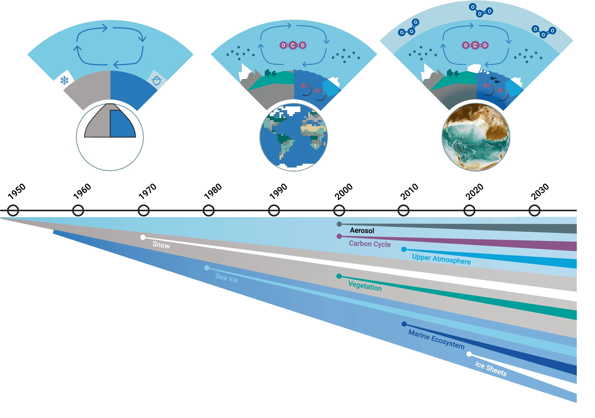
Visual communication
- Uses prediction bands, fan plots, spaghetti plots, and histograms/densities to show how outcomes vary.
- Helps audiences quickly grasp the range and shape of uncertainty.
Numerical summaries
- Provide quantitative measures such as means, medians, IQRs, percentile intervals, and exceedance probabilities.
- Make uncertainty actionable for risk assessment and decision-making.
Verbal statements
- Use calibrated language (“likely,” “high confidence,” “plausible”) to express confidence levels and evidence strength.
- Especially valuable for communication with the public and policymakers.
- Uses prediction bands, fan plots, spaghetti plots, and histograms/densities to show how outcomes vary.
Effective communication blends all three modes to create transparent, honest, and decision-relevant descriptions of model uncertainty.